Finite Markov Decision Processes
Original Source:
Reinforcement Learning: An Introduction Second edition by Richard S. Sutton and Andrew G. Barto
About the Authors:
Richard S. Sutton is a Canadian computer scientist. Currently, he is a distinguished research scientist at DeepMind and a professor of computing science at the University of Alberta. Sutton is considered one of the founding fathers of modern computational reinforcement learning, having several significant contributions to the field, including temporal difference learning and policy gradient methods.
Andrew G. Barto (born c. 1948) is a professor emeritus of computer science at University of Massachusetts Amherst, and chair of the department since January 2007. His main research area is reinforcement learning. He was the supervisor of Sutton during his MS and PhD days.
Here we introduce the problem that we try to solve in the rest of the chapters. For us, this problem defines the field of reinforcement learning: any method that is suited to solving this problem we consider to be a reinforcement learning method. Our objective in this chapter is to describe the reinforcement learning problem in a broad sense. We try to convey the wide range of possible applications that can be framed as reinforcement learning tasks. We also describe mathematically idealized forms of the reinforcement learning problem for which precise theoretical statements can be made. We introduce key elements of the problem’s mathematical structure, such as value functions and Bellman equations. As in all of artificial intelligence, there is a tension between breadth of applicability and mathematical tractability. In this chapter we introduce this tension and discuss some of the trade-offs and challenges that it implies.
The Agent–Environment Interface
The reinforcement learning problem is meant to be a straightforward framing of the problem of learning from interaction to achieve a goal. The learner and decision-maker is called the agent. The thing it interacts with, comprising everything outside the agent, is called the environment. These interact continually, the agent selecting actions and the environment responding to those actions and presenting new situations to the agent. The environment also gives rise to rewards, special numerical values that the agent tries to maximize over time. A complete specification of an environment defines a task , one instance of the reinforcement learning problem.
More specifically, the agent and environment interact at each of a sequence of discrete time steps, \(t = 0, 1, 2, 3, ....\) At each time step \(t\), the agent receives some representation of the environment’s state, \(S_t ∈ S\), where \(S\) is the set of possible states, and on that basis selects an action, \(A_t ∈ A(S_t),\) where \(A(S_t)\) is the set of actions available in state \(S_t\) . One time step later, in part as a consequence of its action, the agent receives a numerical reward , \(R_{t+1} ∈ \mathbb{R}\), and finds itself in a new state, \(S_{t+1}\).
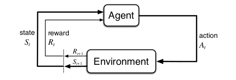
Fig. 39 The agent–environment interaction in reinforcement learning.
At each time step, the agent implements a mapping from states to probabilities of selecting each possible action. This mapping is called the agent’s policy and is denoted \(\pi_t\) , where \(\pi_t(a|s)\) is the probability that \(A_t = a\) if \(S_t = s\). Reinforcement learning methods specify how the agent changes its policy as a result of its experience. The agent’s goal, roughly speaking, is to maximize the total amount of reward it receives over the long run. This framework is abstract and flexible and can be applied to many different problems in many different ways. For example, the time steps need not refer to fixed intervals of real time; they can refer to arbitrary successive stages of decision-making and acting. The actions can be low-level controls, such as the voltages applied to the motors of a robot arm, or high-level decisions, such as whether or not to have lunch or to go to graduate school. Similarly, the states can take a wide variety of forms. They can be completely determined by low-level sensations, such as direct sensor readings, or they can be more high-level and abstract, such as symbolic descriptions of objects in a room. Some of what makes up a state could be based on memory of past sensations or even be entirely mental or subjective. For example, an agent could be in the state of not being sure where an object is, or of having just been surprised in some clearly defined sense. Similarly, some actions might be totally mental or computational. For example, some actions might control what an agent chooses to think about, or where it focuses its attention. In general, actions can be any decisions we want to learn how to make, and the states can be anything we can know that might be useful in making them. In particular, the boundary between agent and environment is not often the same as the physical boundary of a robot’s or animal’s body. Usually, the boundary is drawn closer to the agent than that. For example, the motors and mechanical linkages of a robot and its sensing hardware should usually be considered parts of the environment rather than parts of the agent. Similarly, if we apply the framework to a person or animal, the muscles, skeleton, and sensory organs should be considered part of the environment. Rewards, too, presumably are computed inside the physical bodies of natural and artificial learning systems, but are considered external to the agent.
Note
The general rule we follow is that anything that cannot be changed arbitrarily by the agent is considered to be outside of it and thus part of its environment. We do not assume that everything in the environment is unknown to the agent. For example, the agent often knows quite a bit about how its rewards are computed as a function of its actions and the states in which they are taken. But we always consider the reward computation to be external to the agent because it defines the task facing the agent and thus must be beyond its ability to change arbitrarily. In fact, in some cases the agent may know everything about how its environment works and still face a difficult reinforcement learning task, just as we may know exactly how a puzzle like Rubik’s cube works, but still be unable to solve it. The agent–environment boundary represents the limit of the agent’s absolute control, not of its knowledge.
The agent–environment boundary can be located at different places for different purposes. In a complicated robot, many different agents may be operating at once, each with its own boundary. For example, one agent may make high-level decisions which form part of the states faced by a lower-level agent that implements the high-level decisions. In practice, the agent–environment boundary is determined once one has selected particular states, actions, and rewards, and thus has identified a specific decision-making task of interest. The reinforcement learning framework is a considerable abstraction of the problem of goal-directed learning from interaction. It proposes that whatever the details of the sensory, memory, and control apparatus, and whatever objective one is trying to achieve, any problem of learning goal-directed behavior can be reduced to three signals passing back and forth between an agent and its environment:
one signal to represent the choices made by the agent (the actions)
one signal to represent the basis on which the choices are made (the states)
one signal to define the agent’s goal (the rewards). This framework may not be sufficient to represent all decision-learning problems usefully, but it has proved to be widely useful and applicable.
Of course, the particular states and actions vary greatly from task to task, and how they are represented can strongly affect performance. In reinforcement learning, as in other kinds of learning, such representational choices are at present more art than science. Here we offer some advice and examples regarding good ways of representing states and actions, but our primary focus is on general principles for learning how to behave once the representations have been selected.
Example 1: Bioreactor
Suppose reinforcement learning is being applied to determine moment-by-moment temperatures and stirring rates for a bioreactor (a large vat of nutrients and bacteria used to produce useful chemicals). The actions in such an application might be target temperatures and target stirring rates that are passed to lower-level control systems that, in turn, directly activate heating elements and motors to attain the targets. The states are likely to be thermocouple and other sensory readings, perhaps filtered and delayed, plus symbolic inputs representing the ingredients in the vat and the target chemical. The rewards might be moment-by-moment measures of the rate at which the useful chemical is produced by the bioreactor. Notice that here each state is a list, or vector, of sensor readings and symbolic inputs, and each action is a vector consisting of a target temperature and a stirring rate. It is typical of reinforcement learning tasks to have states and actions with such structured representations. Rewards, on the other hand, are always single numbers.
Example 2: Pick-and-Place Robot
Consider using reinforcement learning to control the motion of a robot arm in a repetitive pick-and-place task. If we want to learn movements that are fast and smooth, the learning agent will have to control the motors directly and have low-latency information about the current positions and velocities of the mechanical linkages. The actions in this case might be the voltages applied to each motor at each joint, and the states might be the latest readings of joint angles and velocities. The reward might be \(+1\) for each object successfully picked up and placed. To encourage smooth movements, on each time step a small, negative reward can be given as a function of the moment-to-moment “jerkiness” of the motion.
Example 3: Recycling Robot
A mobile robot has the job of collecting empty soda cans in an office environment. It has sensors for detecting cans, and an arm and gripper that can pick them up and place them in an onboard bin; it runs on a rechargeable battery. The robot’s control system has components for interpreting sensory information, for navigating, and for controlling the arm and gripper. High-level decisions about how to search for cans are made by a reinforcement learning agent based on the current charge level of the battery. This agent has to decide whether the robot should:
actively search for a can for a certain period of time
remain stationary and wait for someone to bring it a can
head back to its home base to recharge its battery
This decision has to be made either periodically or whenever certain events occur, such as finding an empty can. The agent therefore has three actions, and its state is determined by the state of the battery. The rewards might be zero most of the time, but then become positive when the robot secures an empty can, or large and negative if the battery runs all the way down. In this example, the reinforcement learning agent is not the entire robot. The states it monitors describe conditions within the robot itself, not conditions of the robot’s external environment. The agent’s environment therefore includes the rest of the robot, which might contain other complex decision-making systems, as well as the robot’s external environment.
Goals and Rewards
In reinforcement learning, the purpose or goal of the agent is formalized in terms of a special reward signal passing from the environment to the agent. At each time step, the reward is a simple number, \(R_t ∈ \mathbb{R}\). Informally, the agent’s goal is to maximize the total amount of reward it receives. This means maximizing not immediate reward, but cumulative reward in the long run. We can clearly state this informal idea as the reward hypothesis:
That all of what we mean by goals and purposes can be well thought of as the maximization of the expected value of the cumulative sum of a received scalar signal (called reward).
The use of a reward signal to formalize the idea of a goal is one of the most distinctive features of reinforcement learning.
Although formulating goals in terms of reward signals might at first appear limiting, in practice it has proved to be flexible and widely applicable. The best way to see this is to consider examples of how it has been, or could be, used. For example, to make a robot learn to walk, researchers have provided reward on each time step proportional to the robot’s forward motion. In making a robot learn how to escape from a maze, the reward is often \(−1\) for every time step that passes prior to escape; this encourages the agent to escape as quickly as possible. To make a robot learn to find and collect empty soda cans for recycling, one might give it a reward of zero most of the time, and then a reward of \(+1\) for each can collected. One might also want to give the robot negative rewards when it bumps into things or when somebody yells at it. For an agent to learn to play checkers or chess, the natural rewards are \(+1\) for winning, \(−1\) for losing, and \(0\) for drawing and for all nonterminal positions.
You can see what is happening in all of these examples. The agent always learns to maximize its reward. If we want it to do something for us, we must provide rewards to it in such a way that in maximizing them the agent will also achieve our goals. It is thus critical that the rewards we set up truly indicate what we want accomplished. In particular, the reward signal is not the place to impart to the agent prior knowledge about how to achieve what we want it to do. For example, a chess-playing agent should be rewarded only for actually winning, not for achieving subgoals such taking its opponent’s pieces or gaining control of the center of the board. If achieving these sorts of subgoals were rewarded, then the agent might find a way to achieve them without achieving the real goal. For example, it might find a way to take the opponent’s pieces even at the cost of losing the game. The reward signal is your way of communicating to the robot what you want it to achieve, not how you want it achieved.
Newcomers to reinforcement learning are sometimes surprised that the rewards—which define of the goal of learning—are computed in the environment rather than in the agent. Certainly most ultimate goals for animals are recognized by computations occurring inside their bodies, for example, by sensors for recognizing food, hunger, pain, and pleasure. Nevertheless, as we discussed in the previous section, one can redraw the agent–environment interface in such a way that these parts of the body are considered to be outside of the agent (and thus part of the agent’s environment). For example, if the goal concerns a robot’s internal energy reservoirs, then these are considered to be part of the environment; if the goal concerns the positions of the robot’s limbs, then these too are considered to be part of the environment—that is, the agent’s boundary is drawn at the interface between the limbs and their control systems. These things are considered internal to the robot but external to the learning agent. For our purposes, it is convenient to place the boundary of the learning agent not at the limit of its physical body, but at the limit of its control.
Note
The reason we do this is that the agent’s ultimate goal should be something over which it has imperfect control: it should not be able, for example, to simply decree that the reward has been received in the same way that it might arbitrarily change its actions. Therefore, we place the reward source outside of the agent. This does not preclude the agent from defining for itself a kind of internal reward, or a sequence of internal rewards. Indeed, this is exactly what many reinforcement learning methods do.
Returns
So far we have discussed the objective of learning informally. We have said that the agent’s goal is to maximize the cumulative reward it receives in the long run. How might this be defined formally? If the sequence of rewards received after time step \(t\) is denoted \(R_{t+1}, R_{t+2}, R_{t+3}, . . .,\) then what precise aspect of this sequence do we wish to maximize? In general, we seek to maximize the expected return, where the return \(G_t\) is defined as some specific function of the reward sequence. In the simplest case the return is the sum of the rewards:
where \(T\) is a final time step. This approach makes sense in applications in which there is a natural notion of final time step, that is, when the agent–environment interaction breaks naturally into subsequences, which we call episodes or trials, such as plays of a game, trips through a maze, or any sort of repeated interactions. Each episode ends in a special state called the terminal state, followed by a reset to a standard starting state or to a sample from a standard distribution of starting states. Tasks with episodes of this kind are called episodic tasks. In episodic tasks we sometimes need to distinguish the set of all nonterminal states, denoted \(S\), from the set of all states plus the terminal state, denoted \(S^+\) .
On the other hand, in many cases the agent–environment interaction does not break naturally into identifiable episodes, but goes on continually without limit. For example, this would be the natural way to formulate a continual process-control task, or an application to a robot with a long life span. We call these continuing tasks. The return formulation is problematic for continuing tasks because the final time step would be \(T = \infty\), and the return, which is what we are trying to maximize, could itself easily be infinite. (For example, suppose the agent receives a reward of \(+1\) at each time step.) Thus, here we usually use a definition of return that is slightly more complex conceptually but much simpler mathematically.
The additional concept that we need is that of discounting. According to this approach, the agent tries to select actions so that the sum of the discounted rewards it receives over the future is maximized. In particular, it chooses \(A_t\) to maximize the expected discounted return:
where \(\gamma\) is a parameter, \(0 ≤ \gamma ≤ 1\), called the discount rate.
The discount rate determines the present value of future rewards: a reward received \(k\) time steps in the future is worth only \(\gamma^{k−1}\) times what it would be worth if it were received immediately. If \(\gamma < 1\), the infinite sum has a finite value as long as the reward sequence \(\{R_k\}\) is bounded. If \(\gamma = 0\), the agent is “myopic” in being concerned only with maximizing immediate rewards: its objective in this case is to learn how to choose \(A_t\) so as to maximize only \(R_{t+1}\) . If each of the agent’s actions happened to influence only the immediate reward, not future rewards as well, then a myopic agent could maximize by separately maximizing each immediate reward. But in general, acting to maximize immediate reward can reduce access to future rewards so that the return may actually be reduced. As \(\gamma\) approaches 1, the objective takes future rewards into account more strongly: the agent becomes more farsighted.
Example: Pole-Balancing State

Fig. 40 The pole-balancing task.
The above figure shows a task that served as an early illustration of reinforcement learning. The objective here is to apply forces to a cart moving along a track so as to keep a pole hinged to the cart from falling over. A failure is said to occur if the pole falls past a given angle from vertical or if the cart runs off the track. The pole is reset to vertical after each failure. This task could be treated as episodic, where the natural episodes are the repeated attempts to balance the pole. The reward in this case could be \(+1\) for every time step on which failure did not occur, so that the return at each time would be the number of steps until failure. Alternatively, we could treat pole-balancing as a continuing task, using discounting. In this case the reward would be \(−1\) on each failure and zero at all other times. The return at each time would then be related to \(-\gamma^K\) , where \(K\) is the number of time steps before failure. In either case, the return is maximized by keeping the pole balanced for as long as possible.
Unified Notation for Episodic and Continuing Tasks
In the preceding section we described two kinds of reinforcement learning tasks, one in which the agent–environment interaction naturally breaks down into a sequence of separate episodes (episodic tasks), and one in which it does not (continuing tasks). The former case is mathematically easier because each action affects only the finite number of rewards subsequently received during the episode. Here we consider sometimes one kind of problem and sometimes the other, but often both. It is therefore useful to establish one notation that enables us to talk precisely about both cases simultaneously. To be precise about episodic tasks requires some additional notation. Rather than one long sequence of time steps, we need to consider a series of episodes, each of which consists of a finite sequence of time steps. We number the time steps of each episode starting anew from zero. Therefore, we have to refer not just to \(S_t\) , the state representation at time \(t\), but to \(S_{t,i}\), the state representation at time \(t\) of episode \(i\) (and similarly for \(A_{t,i}, R_{t,i}, \pi_{t,i}, T_i\), etc.). However, it turns out that, when we discuss episodic tasks we will almost never have to distinguish between different episodes. We will almost always be considering a particular single episode, or stating something that is true for all episodes. Accordingly, in practice we will almost always abuse notation slightly by dropping the explicit reference to episode number. That is, we will write \(S_{t}\) to refer to \(S_{t,i}\), and so on.
We need one other convention to obtain a single notation that covers both episodic and continuing tasks. We have defined the return as a sum over a finite number of terms in one case (1) and as a sum over an infinite number of terms in the other (2). These can be unified by considering episode termination to be the entering of a special absorbing state that transitions only to itself and that generates only rewards of zero. For example, consider the state transition diagram:
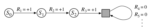
Fig. 41 State Transition diagram
Here the solid square represents the special absorbing state corresponding to the end of an episode. Starting from \(S_0\) , we get the reward sequence \(+1, +1, +1, 0, 0, 0, . . .\). Summing these, we get the same return whether we sum over the first \(T\) rewards (here \(T\) = 3) or over the full infinite sequence. This remains true even if we introduce discounting. Thus, we can define the return, in general, using the convention of omitting episode numbers when they are not needed, and including the possibility that \(\gamma = 1\) if the sum remains defined (e.g., because all episodes terminate). Alternatively, we can also write the return as
including the possibility that \(T = \infty\) or \(\gamma = 1\). We use these conventions throughout the rest of the chapter to simplify notation and to express the close parallels between episodic and continuing tasks.
The Markov Property
In the reinforcement learning framework, the agent makes its decisions as a function of a signal from the environment called the environment’s state. In this section we discuss what is required of the state signal, and what kind of information we should and should not expect it to provide. In particular, we formally define a property of environments and their state signals that is of particular interest, called the Markov property.
Here, by “the state” we mean whatever information is available to the agent. We assume that the state is given by some preprocessing system that is nominally part of the environment. We do not address the issues of constructing, changing, or learning the state signal here. We take this approach not because we consider state representation to be unimportant, but in order to focus fully on the decision-making issues. In other words, our main concern is not with designing the state signal, but with deciding what action to take as a function of whatever state signal is available.
Certainly the state signal should include immediate sensations such as sensory measurements, but it can contain much more than that. State representations can be highly processed versions of original sensations, or they can be complex structures built up over time from the sequence of sensations. For example, we can move our eyes over a scene, with only a tiny spot corresponding to the fovea visible in detail at any one time, yet build up a rich and detailed representation of a scene. Or, more obviously, we can look at an object, then look away, and know that it is still there. We can hear the word “yes” and consider ourselves to be in totally different states depending on the question that came before and which is no longer audible. At a more mundane level, a control system can measure position at two different times to produce a state representation including information about velocity. In all of these cases the state is constructed and maintained on the basis of immediate sensations together with the previous state or some other memory of past sensations. Here, we do not explore how that is done, but certainly it can be and has been done. There is no reason to restrict the state representation to immediate sensations; in typical applications we should expect the state representation to be able to inform the agent of more than that.
On the other hand, the state signal should not be expected to inform the agent of everything about the environment, or even everything that would be useful to it in making decisions. If the agent is playing blackjack, we should not expect it to know what the next card in the deck is. If the agent is answering the phone, we should not expect it to know in advance who the caller is. If the agent is a paramedic called to a road accident, we should not expect it to know immediately the internal injuries of an unconscious victim. In all of these cases there is hidden state information in the environment, and that information would be useful if the agent knew it, but the agent cannot know it because it has never received any relevant sensations. In short, we don’t fault an agent for not knowing something that matters, but only for having known something and then forgotten it!
What we would like, ideally, is a state signal that summarizes past sensations compactly, yet in such a way that all relevant information is retained. This normally requires more than the immediate sensations, but never more than the complete history of all past sensations. A state signal that succeeds in retaining all relevant information is said to be Markov, or to have the Markov property (we define this formally below). For example, a checkers position—the current configuration of all the pieces on the board—would serve as a Markov state because it summarizes everything important about the complete sequence of positions that led to it. Much of the information about the sequence is lost, but all that really matters for the future of the game is retained. Similarly, the current position and velocity of a cannonball is all that matters for its future flight. It doesn’t matter how that position and velocity came about. This is sometimes also referred to as an “independence of path” property because all that matters is in the current state signal; its meaning is independent of the “path,” or history, of signals that have led up to it.
We now formally define the Markov property for the reinforcement learning problem. To keep the mathematics simple, we assume here that there are a finite number of states and reward values. This enables us to work in terms of sums and probabilities rather than integrals and probability densities, but the argument can easily be extended to include continuous states and rewards. Consider how a general environment might respond at time \(t + 1\) to the action taken at time \(t\). In the most general, causal case this response may depend on everything that has happened earlier. In this case the dynamics can be defined only by specifying the complete probability distribution:
for all \(r, s^\prime, A_t\) and all possible values of the past events: \(S_0 , A_0 , R_1 , ..., S_{t−1} ,A_{t−1} , R_t , S_t , A_t\). If the state signal has the Markov property, on the other hand, then the environment’s response at \(t + 1\) depends only on the state and action representations at \(t\), in which case the environment’s dynamics can bedefined by specifying only
for all \(r, s^\prime, S_t, A_t\) . In other words, a state signal has the Markov property, and is a Markov state, if and only if (5) is equal to (4) for all \(s^\prime , r\) and histories, \(S_0 , A_0 , R_1 , ..., S_{t−1} ,A_{t−1} , R_t , S_t , A_t\). In this case, the environment and task as a whole are also said to have the Markov property.
If an environment has the Markov property, then its one-step dynamics (5) enable us to predict the next state and expected next reward given the current state and action. One can show that, by iterating this equation, one can predict all future states and expected rewards from knowledge only of the current state as well as would be possible given the complete history up to the current time. It also follows that Markov states provide the best possible basis for choosing actions. That is, the best policy for choosing actions as a function of a Markov state is just as good as the best policy for choosing actions as a function of complete histories.
Even when the state signal is non-Markov, it is still appropriate to think of the state in reinforcement learning as an approximation to a Markov state. In particular, we always want the state to be a good basis for predicting future rewards and for selecting actions. In cases in which a model of the environment is learned, we also want the state to be a good basis for predicting subsequent states. Markov states provide an unsurpassed basis for doing all of these things. To the extent that the state approaches the ability of Markov states in these ways, one will obtain better performance from reinforcement learning systems. For all of these reasons, it is useful to think of the state at each time step as an approximation to a Markov state, although one should remember that it may not fully satisfy the Markov property.
Note
The Markov property is important in reinforcement learning because decisions and values are assumed to be a function only of the current state. In order for these to be effective and informative, the state representation must be informative. All of the theory presented here assumes Markov state signals. This means that not all the theory strictly applies to cases in which the Markov property does not strictly apply. However, the theory developed for the Markov case still helps us to understand the behavior of the algorithms, and the algorithms can be successfully applied to many tasks with states that are not strictly Markov. A full understanding of the theory of the Markov case is an essential foundation for extending it to the more complex and realistic non-Markov case. Finally, we note that the assumption of Markov state representations is not unique to reinforcement learning but is also present in most, if not all, other approaches to artificial intelligence.
Example: Pole-Balancing State
In the pole-balancing task introduced earlier, a state signal would be Markov if it specified exactly, or made it possible to reconstruct exactly, the position and velocity of the cart along the track, the angle between the cart and the pole, and the rate at which this angle is changing (the angular velocity). In an idealized cart–pole system, this information would be sufficient to exactly predict the future behavior of the cart and pole, given the actions taken by the controller. In practice, however, it is never possible to know this information exactly because any real sensor would introduce some distortion and delay in its measurements. Furthermore, in any real cart–pole system there are always other effects, such as the bending of the pole, the temperatures of the wheel and pole bearings, and various forms of backlash, that slightly affect the behavior of the system. These factors would cause violations of the Markov property if the state signal were only the positions and velocities of the cart and the pole.
However, often the positions and velocities serve quite well as states. Some early studies of learning to solve the pole-balancing task used a coarse state signal that divided cart positions into three regions: right, left, and middle (and similar rough quantizations of the other three intrinsic state variables). This distinctly non-Markov state was sufficient to allow the task to be solved easily by reinforcement learning methods. In fact, this coarse representation may have facilitated rapid learning by forcing the learning agent to ignore fine distinctions that would not have been useful in solving the task.
Example: Draw Poker
In draw poker, each player is dealt a hand of five cards. There is a round of betting, in which each player exchanges some of his cards for new ones, and then there is a final round of betting. At each round, each player must match or exceed the highest bets of the other players, or else drop out (fold). After the second round of betting, the player with the best hand who has not folded is the winner and collects all the bets.
The state signal in draw poker is different for each player. Each player knows the cards in his own hand, but can only guess at those in the other players’ hands. A common mistake is to think that a Markov state signal should include the contents of all the players’ hands and the cards remaining in the deck. In a fair game, however, we assume that the players are in principle unable to determine these things from their past observations. If a player did know them, then she could predict some future events (such as the cards one could exchange for) better than by remembering all past observations.
In addition to knowledge of one’s own cards, the state in draw poker should include the bets and the numbers of cards drawn by the other players. For example, if one of the other players drew three new cards, you may suspect he retained a pair and adjust your guess of the strength of his hand accordingly. The players’ bets also influence your assessment of their hands. In fact, much of your past history with these particular players is part of the Markov state. Does Ellen like to bluff, or does she play conservatively? Does her face or demeanor provide clues to the strength of her hand? How does Joe’s play change when it is late at night, or when he has already won a lot of money?
Although everything ever observed about the other players may have an effect on the probabilities that they are holding various kinds of hands, in practice this is far too much to remember and analyze, and most of it will have no clear effect on one’s predictions and decisions. Very good poker players are adept at remembering just the key clues, and at sizing up new players quickly, but no one remembers everything that is relevant. As a result, the state representations people use to make their poker decisions are undoubtedly non-Markov, and the decisions themselves are presumably imperfect. Nevertheless, people still make very good decisions in such tasks. We conclude that the inability to have access to a perfect Markov state representation is probably not a severe problem for a reinforcement learning agent.
Markov Decision Processes
A reinforcement learning task that satisfies the Markov property is called a Markov decision process, or MDP. If the state and action spaces are finite, then it is called a finite Markov decision process (finite MDP). Finite MDPs are particularly important to the theory of reinforcement learning. We treat them extensively throughout this chapter; they are all you need to understand \(90\%\) of modern reinforcement learning.
A particular finite MDP is defined by its state and action sets and by the one-step dynamics of the environment. Given any state and action \(s\) and \(a\), the probability of each possible pair of next state and reward, \(s^\prime , r\), is denoted
These quantities completely specify the dynamics of a finite MDP. Most of the theory we present here implicitly assumes the environment is a finite MDP. Given the dynamics as specified by (6), one can compute anything else one might want to know about the environment, such as the expected rewards for state–action pairs,
the state-transition probabilities,
and the expected rewards for state–action–next-state triples,
Example: Recycling Robot MDP
The recycling robot can be turned into a simple example of an MDP by simplifying it and providing some more details. (Our aim is to produce a simple example, not a particularly realistic one.) Recall that the agent makes a decision at times determined by external events (or by other parts of the robot’s control system). At each such time the robot decides whether it should
actively search for a can
remain stationary and wait for someone to bring it a can
go back to home base to recharge its battery.
Suppose the environment works as follows. The best way to find cans is to actively search for them, but this runs down the robot’s battery, whereas waiting does not. Whenever the robot is searching, the possibility exists that its battery will become depleted. In this case the robot must shut down and wait to be rescued (producing a low reward).
The agent makes its decisions solely as a function of the energy level of the battery. It can distinguish two levels, high and low, so that the state set is \(S = \{high, low\}\). Let us call the possible decisions—the agent’s actions— \(\{wait, search, recharge\}\). When the energy level is high, recharging would always be foolish, so we do not include it in the action set for this state. The agent’s action sets are
If the energy level is high, then a period of active search can always be completed without risk of depleting the battery. A period of searching that begins with a high energy level leaves the energy level high with probability \(\alpha\) and reduces it to low with probability \(1- \alpha\). On the other hand, a period of searching undertaken when the energy level is low leaves it low with probability \(\beta\) and depletes the battery with probability \(1- \beta\). In the latter case, the robot must be rescued, and the battery is then recharged back to high. Each can collected by the robot counts as \(+1\) reward, whereas a reward of \(−3\) results whenever the robot has to be rescued. Let \(r_{search}\) and \(r_{wait} \), with \(r_{search} > r_{wait} \) , respectively denote the expected number of cans the robot will collect (and hence the expected reward) while searching and while waiting. Finally, to keep things simple, suppose that no cans can be collected during a run home for recharging, and that no cans can be collected on a step in which the battery is depleted. This system is then a finite MDP, and we can write down the transition probabilities and the expected rewards, as in the below table
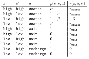
Fig. 42 Transition probabilities and expected rewards for the finite MDP of the recycling robot example. There is a row for each possible combination of current state, \(s\), next state, \(s^\prime\) , and action possible in the current state, \(a ∈ A(s)\).
A transition graph is a useful way to summarize the dynamics of a finite MDP. Figure below shows the transition graph for the recycling robot example. There are two kinds of nodes:
state nodes
action nodes
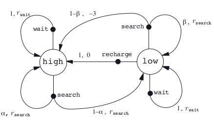
Fig. 43 Transition graph for the recycling robot example
There is a state node for each possible state (a large open circle labeled by the name of the state), and an action node for each state–action pair (a small solid circle labeled by the name of the action and connected by a line to the state node). Starting in state \(s\) and taking action \(a\) moves you along the line from state node \(s\) to action node \((s, a)\). Then the environment responds with a transition to the next state’s node via one of the arrows leaving action node \((s, a)\). Each arrow corresponds to a triple \((s, s^\prime, a)\), where \(s^\prime\) is the next state, and we label the arrow with the transition probability, \(p(s^\prime |s, a)\), and the expected reward for that transition \(r(s, a, s^\prime)\). Note that the transition probabilities labeling the arrows leaving an action node always sum to \(1\).
Value Functions
Almost all reinforcement learning algorithms involve estimating value functions—functions of states (or of state–action pairs) that estimate how good it is for the agent to be in a given state (or how good it is to perform a given action in a given state). The notion of “how good” here is defined in terms of future rewards that can be expected, or, to be precise, in terms of expected return. Of course the rewards the agent can expect to receive in the future depend on what actions it will take. Accordingly, value functions are defined with respect to particular policies. Recall that a policy, \(\pi\), is a mapping from each state, \(s ∈ S\), and action, \(a ∈ A(s)\), to the probability \(\pi(a|s)\) of taking action \(a\) when in state \(s\). Informally, the value of a state \(s\) under a policy \(\pi\), denoted \(v_\pi(s)\), is the expected return when starting in \(s\) and following \(\pi\) thereafter. For MDPs, we can define \(v_\pi(s)\) formally as
where \(E_{\pi}[·]\) denotes the expected value of a random variable given that the agent follows policy \(\pi\), and \(t\) is any time step. Note that the value of the terminal state, if any, is always zero. We call the function \(v_{\pi}\) the state-value function for policy \(\pi\).
Similarly, we define the value of taking action \(a\) in state \(s\) under a policy \(\pi\), denoted \(q_\pi(s, a)\), as the expected return starting from \(s\), taking the action \(a\), and thereafter following policy \(\pi\):
We call \(q_\pi\) the action-value function for policy \(\pi\).
The value functions \(v_\pi\) and \(q_\pi\) can be estimated from experience. For example, if an agent follows policy \(\pi\) and maintains an average, for each state encountered, of the actual returns that have followed that state, then the average will converge to the state’s value, \(v_\pi(s)\), as the number of times that state is encountered approaches infinity. If separate averages are kept for each action taken in a state, then these averages will similarly converge to the action values, \(q_\pi(s,a)\). We call estimation methods of this kind Monte Carlo methods because they involve averaging over many random samples of actual returns. Of course, if there are very many states, then it may not be practical to keep separate averages for each state individually. Instead, the agent would have to maintain \(v_\pi\) and \(q_\pi\) as parameterized functions and adjust the parameters to better match the observed returns. This can also produce accurate estimates, although much depends on the nature of the parameterized function approximator.
A fundamental property of value functions used throughout reinforcement learning and dynamic programming is that they satisfy particular recursive relationships. For any policy \(\pi\) and any state \(s\), the following consistency condition holds between the value of \(s\) and the value of its possible successor states:
where it is implicit that the actions, a, are taken from the set \(A(s)\), the next states, \(s^\prime\), are taken from the set \(S\) (or from \(S^+\) in the case of an episodic problem), and the rewards, \(r\), are taken from the set \(R\). Note also how in the last equation we have merged the two sums, one over all the values of \(s^\prime\) and the other over all values of \(r\), into one sum over all possible values of both. We will use this kind of merged sum often to simplify formulas. Note how the final expression can be read very easily as an expected value. It is really a sum over all values of the three variables, \(a\), \(s^\prime\) , and \(r\).
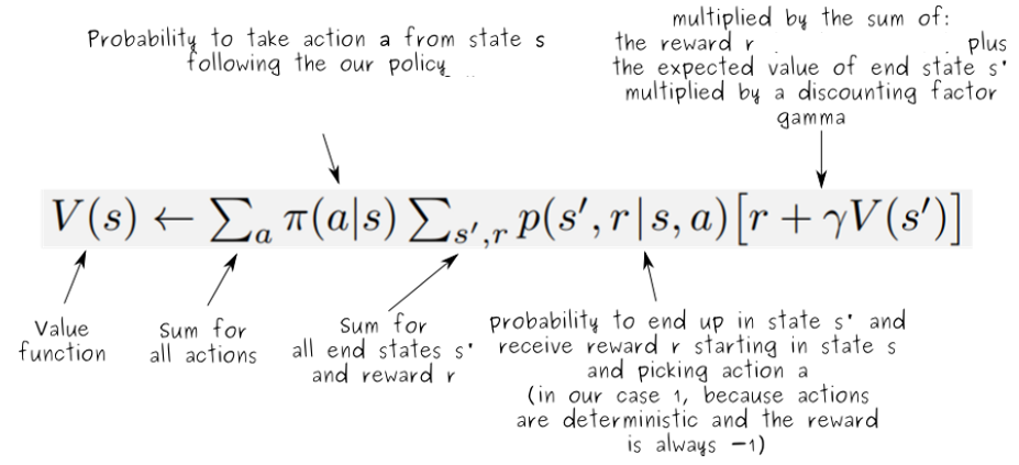
Note
For each triple, we compute its probability, \(\pi(a|s)p(s^\prime, r|s,a)\) i.e probability \(\pi(a|s)\) of taking action \(a\) when in state \(s\) and given any state & action(\(s, a\)) the probability of each possible pair of next state and reward, \((s′,r)\); weight the quantity in brackets by that probability, then sum over all possibilities to get an expected value.
Equation (12) is the Bellman equation for \(v_\pi\). It expresses a relationship between the value of a state and the values of its successor states. Think of looking ahead from one state to its possible successor states, as suggested by the figure below. Each open circle represents a state and each solid circle represents a state–action pair. Starting from state \(s\), the root node at the top, the agent could take any of some set of actions—three are shown in Figure(a). From each of these, the environment could respond with one of several next states, \(s^\prime\) , along with a reward, \(r\). The Bellman equation (12) averages over all the possibilities, weighting each by its probability of occurring. It states that the value of the start state must equal the (discounted) value of the expected next state, plus the reward expected along the way.
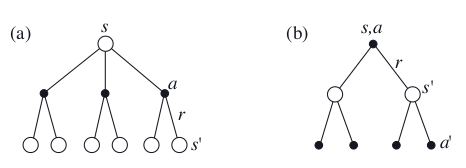
Fig. 45 Backup diagrams for (a) \(v_\pi\) and (b) \(q_\pi\)
The value function \(v_\pi\)is the unique solution to its Bellman equation. We show in subsequent chapters how this Bellman equation forms the basis of a number of ways to compute, approximate, and learn \(v_\pi\) . We call diagrams like those shown in the above figure as backup diagrams because they diagram relationships that form the basis of the update or backup operations that are at the heart of reinforcement learning methods. These operations transfer value information back to a state (or a state–action pair) from its successor states (or state–action pairs). We use backup diagrams throughout the chapter to provide graphical summaries of the algorithms we discuss. (Note that unlike transition graphs, the state nodes of backup diagrams do not necessarily represent distinct states; for example, a state might be its own successor. We also omit explicit arrowheads because time always flows downward in a backup diagram.)
Example: Gridworld
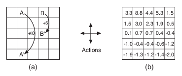
Fig. 46 Grid example: (a) exceptional reward dynamics; (b) state-value function for the equiprobable random policy.
The above figure uses a rectangular grid to illustrate value functions for a simple finite MDP. The cells of the grid correspond to the states of the environment. At each cell, four actions are possible: north, south, east, and west, which deterministically cause the agent to move one cell in the respective direction on the grid. Actions that would take the agent off the grid leave its location unchanged, but also result in a reward of \(−1\). Other actions result in a reward of \(0\), except those that move the agent out of the special states \(A\) and \(B\). From state \(A\), all four actions yield a reward of \(+10\) and take the agent to \(A^\prime\) . From state \(B\), all actions yield a reward of \(+5\) and take the agent to \(B^\prime\).
Suppose the agent selects all four actions with equal probability in all states. Figure(b) shows the value function, \(v_\pi\) , for this policy, for the discounted reward case with \(\gamma = 0.9\). This value function was computed by solving the system of equations (12). Notice the negative values near the lower edge; these are the result of the high probability of hitting the edge of the grid there under the random policy. State \(A\) is the best state to be in under this policy, but its expected return is less than \(10\), its immediate reward, because from \(A\) the agent is taken to \(A^\prime\) , from which it is likely to run into the edge of the grid. State \(B\), on the other hand, is valued more than \(5\), its immediate reward, because from \(B\) the agent is taken to \(B^\prime\) , which has a positive value. From \(B^\prime\) the expected penalty (negative reward) for possibly running into an edge is more than compensated for by the expected gain for possibly stumbling onto \(A\) or \(B\).
Calculation:
The last calculation requires some explanation:
\(0.9*(8.8+1.5)\) because \(\gamma = 0.9, r = 0\) if agent is not off grid and not transitioning from special states \(A\) or \(B\), and \(v(s^\prime)\) is \(8.8\) and \(1.5\) for a left and down move respectively.
\((-1+0.9*3.3)*2\) because \(r = -1\) if agent steps off grid (AKA left or up move), \(0.9\) because that’s \(\gamma\), \(3.3\) because \(v(s^\prime) = v(s)\) as agent remains in its previous state if it steps off grid. Multiplied by \(2\) because there are \(2\) possibilities(left/up move) to for agent to step off grid.
Dividing the sum of part 1 and 2 by \(1/4\) because \(\pi(a|s) = 1/4\) for all actions.
Example: Golf
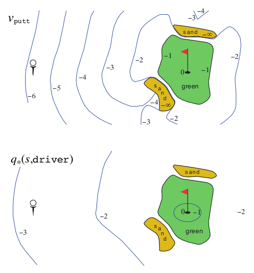
Fig. 47 A golf example: the state-value function for putting (above) and the optimal action-value function for using the driver (below).
To formulate playing a hole of golf as a reinforcement learning task, we count a penalty (negative reward) of \(−1\) for each stroke until we hit the ball into the hole. The state is the location of the ball. The value of a state is the negative of the number of strokes to the hole from that location. Our actions are how we aim and swing at the ball, of course, and which club we select. Let us take the former as given and consider just the choice of club, which we assume is either a putter or a driver. The upper part of the above figure shows a possible state-value function, \(v_{putt}(s)\), for the policy that always uses the putter. The terminal state in-the-hole has a value of \(0\). From anywhere on the green we assume we can make a putt; these states have value \(−1\). Off the green we cannot reach the hole by putting, and the value is greater. If we can reach the green from a state by putting, then that state must have value one less than the green’s value, that is, \(−2\). For simplicity, let us assume we can putt very precisely and deterministically, but with a limited range. This gives us the sharp contour line labeled \(−2\) in the figure; all locations between that line and the green require exactly two strokes to complete the hole. Similarly, any location within putting range of the \(−2\) contour line must have a value of \(−3\), and so on to get all the contour lines shown in the figure. Putting doesn’t get us out of sand traps, so they have a value of \(-\infty\). Overall, it takes us six strokes to get from the tee to the hole by putting.
Optimal Value Functions
Solving a reinforcement learning task means, roughly, finding a policy that achieves a lot of reward over the long run. For finite MDPs, we can precisely define an optimal policy in the following way. Value functions define a partial ordering over policies. A policy \(\pi\) is defined to be better than or equal to a policy \(\pi^\prime\) if its expected return is greater than or equal to that of \(\pi^\prime\) for all states. In other words, \(\pi ≥ \pi^\prime\) if and only if \(v_\pi(s) ≥ v_\pi^{\prime}(s)\) for all \(s ∈ S\). There is always at least one policy that is better than or equal to all other policies. This is an optimal policy. Although there may be more than one, we denote all the optimal policies by \(\pi_*\) . They share the same state-value function, called the optimal state-value function, denoted \(v_*\) , and defined as
for all \(s ∈ S\)
Optimal policies also share the same optimal action-value function, denoted \(q_*\) , and defined as
for all \(s ∈ S\) and \(a ∈ A(s)\). For the state–action pair \((s, a)\), this function gives the expected return for taking action \(a\) in state \(s\) and thereafter following an optimal policy. Thus, we can write \(q_*\) in terms of \(v_*\) as follows:
Example: Optimal Value Functions for Golf
The lower part of Figure in the golf example shows the contours of a possible optimal action-value function \(q_*(s, driver)\). These are the values of each state if we first play a stroke with the driver and afterward select either the driver or the putter, whichever is better. The driver enables us to hit the ball farther, but with less accuracy. We can reach the hole in one shot using the driver only if we are already very close; thus the \(−1\) contour for \(q_*(s, driver)\) covers only a small portion of the green. If we have two strokes, however, then we can reach the hole from much farther away, as shown by the \(−2\) contour. In this case we don’t have to drive all the way to within the small \(−1\) contour, but only to anywhere on the green; from there we can use the putter. The optimal action-value function gives the values after committing to a particular first action, in this case, to the driver, but afterward using whichever actions are best. The \(−3\) contour is still farther out and includes the starting tee. From the tee, the best sequence of actions is two drives and one putt, sinking the ball in three strokes.
Because \(v_*\) is the value function for a policy, it must satisfy the self- consistency condition given by the Bellman equation for state values (12). Because it is the optimal value function, however, \(v_*\) ’s consistency condition can be written in a special form without reference to any specific policy. This is the Bellman equation for \(v_*\) , or the Bellman optimality equation. Intuitively, the Bellman optimality equation expresses the fact that the value of a state under an optimal policy must equal the expected return for the best action from that state:
The last two equations are two forms of the Bellman optimality equation for \(v_*\). The Bellman optimality equation for \(q_*\) is
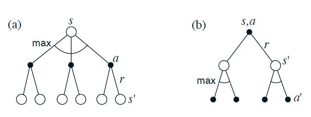
Fig. 48 Backup diagrams for (a) \(v_*\) and (b) \(q_*\)
The backup diagrams above show graphically the spans of future states and actions considered in the Bellman optimality equations for \(v_*\) and \(q_*\). These are the same as the backup diagrams for \(v\) and \(q\) except that arcs have been added at the agent’s choice points to represent that the maximum over that choice is taken rather than the expected value given some policy. Figure(a) graphically represents the Bellman optimality equation (16).
For finite MDPs, the Bellman optimality equation (16) has a unique solution independent of the policy. The Bellman optimality equation is actually a system of equations, one for each state, so if there are N states, then there are N equations in N unknowns. If the dynamics of the environment are known \((p(s^\prime; r|s, a))\), then in principle one can solve this system of equations for \(v_*\) using any one of a variety of methods for solving systems of nonlinear equations. One can solve a related set of equations for \(q_*\).
Once one has \(v_*\), it is relatively easy to determine an optimal policy. For each state \(s\), there will be one or more actions at which the maximum is obtained in the Bellman optimality equation. Any policy that assigns nonzero probability only to these actions is an optimal policy. You can think of this as a one-step search. If you have the optimal value function,\(v_*\), then the actions that appear best after a one-step search will be optimal actions. Another way of saying this is that any policy that is greedy with respect to the optimal evaluation function \(v_*\) is an optimal policy. The term greedy is used in computer science to describe any search or decision procedure that selects alternatives based only on local or immediate considerations, without considering the possibility that such a selection may prevent future access to even better alternatives. Consequently, it describes policies that select actions based only on their short-term consequences. The beauty of \(v_*\) is that if one uses it to evaluate the short-term consequences of actions– specifically, the one-step consequences– then a greedy policy is actually optimal in the longterm sense in which we are interested because \(v_*\) already takes into account the reward consequences of all possible future behavior. By means of \(v_*\), the optimal expected long-term return is turned into a quantity that is locally and immediately available for each state. Hence, a one-step-ahead search yields the long-term optimal actions.
Having \(q_*\) makes choosing optimal actions still easier. With \(q_*\), the agent does not even have to do a one-step-ahead search: for any state s, it can simply find any action that maximizes \(q_*(s, a)\). The action-value function effectively caches the results of all one-step-ahead searches. It provides the optimal expected long-term return as a value that is locally and immediately available for each state{action pair. Hence, at the cost of representing a function of state{action pairs, instead of just of states, the optimal action-value function allows optimal actions to be selected without having to know anything about possible successor states and their values, that is, without having to know anything about the environment’s dynamics.
Example: Bellman Optimality Equations for the Recycling Robot
Using (17), we can explicitly give the Bellman optimality equation for the recycling robot example. To make things more compact, we abbreviate the states high and low, and the actions search, wait, and recharge respectively by h, l, s, w, and re. Since there are only two states, the Bellman optimality equation consists of two equations. The equation for \(v_*(h)\) can be written as follows:
Following the same procedure for \(v_*(l)\) yields the equation
For any choice of \(r_s, r_w, \alpha, \beta\) and \(\gamma\), with \(0 \leq \gamma \leq 1, 0 \leq \alpha, \beta \leq 1\), there is exactly one pair of numbers, \(v_*(h)\) and \(v_*(l)\), that simultaneously satisfy these two nonlinear equations.
Example: Solving the Gridworld
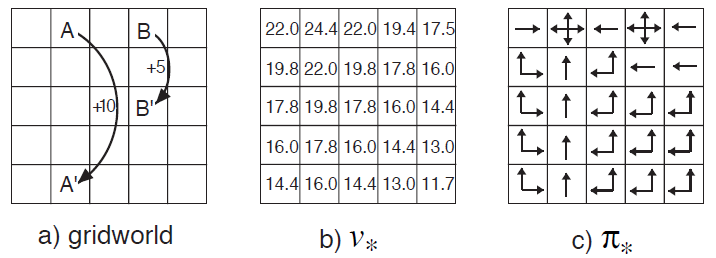
Fig. 49 Optimal solutions to the gridworld example.
Suppose we solve the Bellman equation for \(v_*\) for the simple grid task introduced earlier. Recall that state \(A\) is followed by a reward of \(+10\) and transition to state \(A^\prime\), while state \(B\) is followed by a reward of \(+5\) and transition to state \(B^\prime\). Figure(b) shows the optimal value function, and Figure(c) shows the corresponding optimal policies. Where there are multiple arrows in a cell, any of the corresponding actions is optimal.
Explicitly solving the Bellman optimality equation provides one route to finding an optimal policy, and thus to solving the reinforcement learning problem. However, this solution is rarely directly useful. It is akin to an exhaustive search, looking ahead at all possibilities, computing their probabilities of occurrence and their desirabilities in terms of expected rewards. This solution relies on at least three assumptions that are rarely true in practice: (1) we accurately know the dynamics of the environment; (2) we have enough computational resources to complete the computation of the solution; and (3) the Markov property. For the kinds of tasks in which we are interested, one is generally not able to implement this solution exactly because various combinations of these assumptions are violated. For example, although the first and third assumptions present no problems for the game of backgammon, the second is a major impediment. Since the game has about \(10^{20}\) states, it would take thousands of years on today’s fastest computers to solve the Bellman equation for \(v_*\), and the same is true for finding \(q_*\). In reinforcement learning one typically has to settle for approximate solutions.
Many different decision-making methods can be viewed as ways of approximately solving the Bellman optimality equation. For example, heuristic search methods can be viewed as expanding the right-hand side of (17) several times, up to some depth, forming a “tree” of possibilities, and then using a heuristic evaluation function to approximate \(v_*\) at the “leaf” nodes. (Heuristic search methods such as \(A^*\) are almost always based on the episodic case.) The methods of dynamic programming can be related even more closely to the Bellman optimality equation. Many reinforcement learning methods can be clearly understood as approximately solving the Bellman optimality equation, using actual experienced transitions in place of knowledge of the expected transitions. We consider a variety of such methods in the following chapters.
Optimality and Approximation
We have defined optimal value functions and optimal policies. Clearly, an agent that learns an optimal policy has done very well, but in practice this rarely happens. For the kinds of tasks in which we are interested, optimal policies can be generated only with extreme computational cost. A well-defined notion of optimality organizes the approach to learning we describe here and provides a way to understand the theoretical properties of various learning algorithms, but it is an ideal that agents can only approximate to varying degrees. As we discussed above, even if we have a complete and accurate model of the environment’s dynamics, it is usually not possible to simply compute an optimal policy by solving the Bellman optimality equation. For example, board games such as chess are a tiny fraction of human experience, yet large, custom-designed computers still cannot compute the optimal moves. A critical aspect of the problem facing the agent is always the computational power available to it, in particular, the amount of computation it can perform in a single time step.
The memory available is also an important constraint. A large amount of memory is often required to build up approximations of value functions, policies, and models. In tasks with small, definite state sets, it is possible to form these approximations using arrays or tables with one entry for each state (or state-action pair). This we call the tabular case, and the corresponding methods we call tabular methods. In many cases of practical interest, however, there are far more states than could possibly be entries in a table. In these cases the functions must be approximated, using some sort of more compact parameterized function representation.
Our framing of the reinforcement learning problem forces us to settle for approximations. However, it also presents us with some unique opportunities for achieving useful approximations. For example, in approximating optimal behavior, there may be many states that the agent faces with such a low probability that selecting suboptimal actions for them has little impact on the amount of reward the agent receives. Tesauro’s backgammon player, for example, plays with exceptional skill even though it might make very bad decisions on board configurations that never occur in games against experts. In fact, it is possible that TD-Gammon makes bad decisions for a large fraction of the game’s state set. The on-line nature of reinforcement learning makes it possible to approximate optimal policies in ways that put more effort into learning to make good decisions for frequently encountered states, at the expense of less effort for infrequently encountered states. This is one key property that distinguishes reinforcement learning from other approaches to approximately solving MDPs.
Summary
Let us summarize the elements of the reinforcement learning problem that we have presented in this chapter. Reinforcement learning is about learning from interaction how to behave in order to achieve a goal. The reinforcement learning agent and its environment interact over a sequence of discrete time steps. The specification of their interface defines a particular task: the actions are the choices made by the agent; the states are the basis for making the choices; and the rewards are the basis for evaluating the choices. Everything inside the agent is completely known and controllable by the agent; everything outside is incompletely controllable but may or may not be completely known. A policy is a stochastic rule by which the agent selects actions as a function of states. The agent’s objective is to maximize the amount of reward it receives over time.
The return is the function of future rewards that the agent seeks to maximize. It has several different definitions depending upon the nature of the task and whether one wishes to discount delayed reward. The undiscounted formulation is appropriate for episodic tasks, in which the agent{environment interaction breaks naturally into episodes; the discounted formulation is appropriate for continuing tasks, in which the interaction does not naturally break into episodes but continues without limit.
An environment satisfies the Markov property if its state signal compactly summarizes the past without degrading the ability to predict the future. This is rarely exactly true, but often nearly so; the state signal should be chosen or constructed so that the Markov property holds as nearly as possible. Here we assume that this has already been done and focus on the decisionmaking problem: how to decide what to do as a function of whatever state signal is available. If the Markov property does hold, then the environment is called a Markov decision process (MDP). A finite MDP is an MDP with finite state and action sets. Most of the current theory of reinforcement learning is restricted to finite MDPs, but the methods and ideas apply more generally.
A policy’s value functions assign to each state, or state{action pair, the expected return from that state, or state{action pair, given that the agent uses the policy. The optimal value functions assign to each state, or state{action pair, the largest expected return achievable by any policy. A policy whose value functions are optimal is an optimal policy. Whereas the optimal value functions for states and state{action pairs are unique for a given MDP, there can be many optimal policies. Any policy that is greedy with respect to the optimal value functions must be an optimal policy. The Bellman optimality equations are special consistency condition that the optimal value functions must satisfy and that can, in principle, be solved for the optimal value functions, from which an optimal policy can be determined with relative ease.
A reinforcement learning problem can be posed in a variety of different ways depending on assumptions about the level of knowledge initially available to the agent. In problems of complete knowledge, the agent has a complete and accurate model of the environment’s dynamics. If the environment is an MDP, then such a model consists of the one-step transition probabilities and expected rewards for all states and their allowable actions. In problems of incomplete knowledge, a complete and perfect model of the environment is not available.
Even if the agent is typically unable to perform enough computation per time step to fully use it. The memory available is also an important constraint. Memory may be required to build up accurate approximations of value functions, policies, and models. In most cases of practical interest there are far more states than could possibly be entries in a table, and approximations must be made.
A well-defined notion of optimality organizes the approach to learning we describe here and provides a way to understand the theoretical properties of various learning algorithms, but it is an ideal that reinforcement learning agents can only approximate to varying degrees. In reinforcement learning we are very much concerned with cases in which optimal solutions cannot be found but must be approximated in some way.