Neural Networks as Universal Approximators
Original Source:
Most materials are from A visual proof that neural nets can compute any function by Michael Nielsen. Few materials are of my own
About the Authors:
Michael Aaron Nielsen (born January 4, 1974) is a quantum physicist, science writer, and computer programming researcher living in San Francisco. In 2004 Nielsen was characterized as Australia’s “youngest academic” and secured a Federation Fellowship at the University of Queensland; the fellowship was for five years. He worked at the Los Alamos National Laboratory, as the Richard Chace Tolman Prize Fellow at Caltech, and a Senior Faculty Member at the Perimeter Institute for Theoretical Physics. Nielsen obtained his PhD in physics in 1998 at the University of New Mexico.
With Isaac Chuang he is the co-author of a popular textbook on quantum computing. As of December 2019, the book was cited more than 36,000 times.
In 2007, Nielsen announced a marked shift in his field of research: from quantum information and computation to “the development of new tools for scientific collaboration and publication”. This work, for which he gave up a tenured academic position, includes “massively collaborative mathematics” projects like the Polymath project with Timothy Gowers. Besides writing books and essays, he has also given talks about Open Science. He was a member of the Working Group on Open Data in Science at the Open Knowledge Foundation.
Introduction
One of the most striking facts about neural networks is that they can compute any function at all. That is, suppose someone hands you some complicated, wiggly function, \(f(x)\):
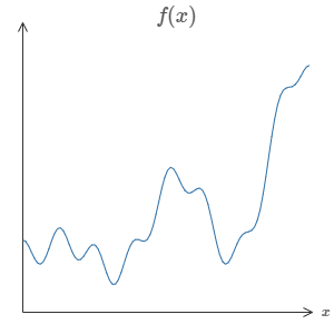
Fig. 8 \(f(x)\)
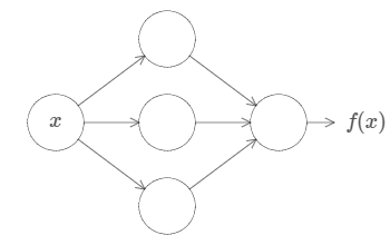
No matter what the function, there is guaranteed to be a neural network so that for every possible input, \(x\), the value \(f(x)\) (or some close approximation) is output from the network, e.g.:
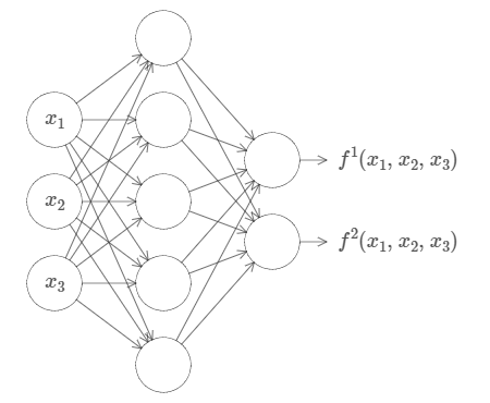
This result holds even if the function has many inputs, \(f=f(x_1,…,x_m)\), and many outputs. For instance, here’s a network computing a function with \(m=3\) inputs and \(n=2\) outputs:
This result tells us that neural networks have a kind of universality. No matter what function we want to compute, we know that there is a neural network which can do the job.
What’s more, this universality theorem holds even if we restrict our networks to have just a single layer intermediate between the input and the output neurons - a so-called single hidden layer. So even very simple network architectures can be extremely powerful.
The universality theorem is well known by people who use neural networks. But why it’s true is not so widely understood. Most of the explanations available are quite technical. For instance, one of the original papers proving the result did so using the Hahn-Banach theorem, the Riesz Representation theorem, and some Fourier analysis. If you’re a mathematician the argument is not difficult to follow, but it’s not so easy for most people. That’s a pity, since the underlying reasons for universality are simple and beautiful.
In this chapter I give a simple and mostly visual explanation of the universality theorem. We’ll go step by step through the underlying ideas. You’ll understand why it’s true that neural networks can compute any function. You’ll understand some of the limitations of the result. And you’ll understand how the result relates to deep neural networks.
Universality theorems are a commonplace in computer science, so much so that we sometimes forget how astonishing they are. But it’s worth reminding ourselves: the ability to compute an arbitrary function is truly remarkable. Almost any process you can imagine can be thought of as function computation. Consider the problem of naming a piece of music based on a short sample of the piece. That can be thought of as computing a function. Or consider the problem of translating a Chinese text into English. Again, that can be thought of as computing a function. Or consider the problem of taking an mp4 movie file and generating a description of the plot of the movie, and a discussion of the quality of the acting. Again, that can be thought of as a kind of function computation. Universality means that, in principle, neural networks can do all these things and many more.
Of course, just because we know a neural network exists that can (say) translate Chinese text into English, that doesn’t mean we have good techniques for constructing or even recognizing such a network. This limitation applies also to traditional universality theorems for models such as Boolean circuits. Neural networks have powerful algorithms for learning functions. That combination of learning algorithms \(+\) universality is an attractive mix. Here, we focus on universality, and what it means.
Two caveats
Before explaining why the universality theorem is true, I want to mention two caveats to the informal statement “a neural network can compute any function”.
First, this doesn’t mean that a network can be used to exactly compute any function. Rather, we can get an approximation that is as good as we want. By increasing the number of hidden neurons we can improve the approximation. For instance, earlier I illustrated a network computing some function \(f(x)\) using three hidden neurons. For most functions only a low-quality approximation will be possible using three hidden neurons. By increasing the number of hidden neurons (say, to five) we can typically get a better approximation:
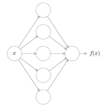
And we can do still better by further increasing the number of hidden neurons.
To make this statement more precise, suppose we’re given a function \(f(x)\) which we’d like to compute to within some desired accuracy \(\epsilon > 0\). The guarantee is that by using enough hidden neurons we can always find a neural network whose output \(g(x)\) satisfies \(|g(x)−f(x)|<\epsilon\), for all inputs \(x\). In other words, the approximation will be good to within the desired accuracy for every possible input.
The second caveat is that the class of functions which can be approximated in the way described are the continuous functions. If a function is discontinuous, i.e., makes sudden, sharp jumps, then it won’t in general be possible to approximate using a neural net. This is not surprising, since our neural networks compute continuous functions of their input. However, even if the function we’d really like to compute is discontinuous, it’s often the case that a continuous approximation is good enough. If that’s so, then we can use a neural network. In practice, this is not usually an important limitation.
Summing up, a more precise statement of the universality theorem is that neural networks with a single hidden layer can be used to approximate any continuous function to any desired precision. In this chapter we’ll actually prove a slightly weaker version of this result, using two hidden layers instead of one. In the problems I’ll briefly outline how the explanation can, with a few tweaks, be adapted to give a proof which uses only a single hidden layer.
Universality with one input and one output
To understand why the universality theorem is true, let’s start by understanding how to construct a neural network which approximates a function with just one input and one output:
Fig. 12 \(f(x)\)
It turns out that this is the core of the problem of universality. Once we’ve understood this special case it’s actually pretty easy to extend to functions with many inputs and many outputs.
To build insight into how to construct a network to compute \(f\), let’s start with a network containing just a single hidden layer, with two hidden neurons and an output layer containing a single output neuron:
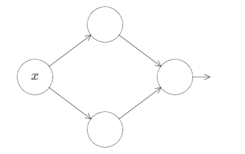
Fig. 13 A network containing just a single hidden layer, with two hidden neurons and an output layer containing a single output neuron
To get a feel for how components in the network work, let’s focus on the top hidden neuron.
Fig. 14 What’s being computed by the hidden neuron is \(σ(wx+b)\), where \(σ(z)≡1/(1+e^{−z})\) is the sigmoid function. As the bias \(b\) increases the graph moves to the left, but its shape doesn’t change and as the bias decreases the graph moves to the right, but, again, its shape doesn’t change. As we decrease the weight, the curve broadens out and if we increase the weight up past \(w=100\), the curve gets steeper, until eventually it begins to look like a step function.
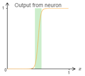
We can simplify our analysis quite a bit by increasing the weight so much that the output really is a step function, to a very good approximation. Below I’ve plotted the output from the top hidden neuron when the weight is \(w=999\).
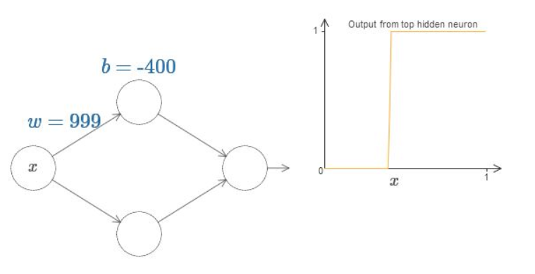
Fig. 15 Output as a step function
It’s actually quite a bit easier to work with step functions than general sigmoid functions. The reason is that in the output layer we add up contributions from all the hidden neurons. It’s easy to analyze the sum of a bunch of step functions, but rather more difficult to reason about what happens when you add up a bunch of sigmoid shaped curves. And so it makes things much easier to assume that our hidden neurons are outputting step functions. More concretely, we do this by fixing the weight w to be some very large value, and then setting the position of the step by modifying the bias. Of course, treating the output as a step function is an approximation, but it’s a very good approximation, and for now we’ll treat it as exact. I’ll come back later to discuss the impact of deviations from this approximation.
At what value of \(x\) does the step occur? Put another way, how does the position of the step depend upon the weight and bias? With a little work you should be able to convince yourself that the position of the step is proportional to \(b\), and inversely proportional to \(w\). In fact, the step is at position \(s=−b/w\), as you can see by modifying the weight and bias in the following diagram:
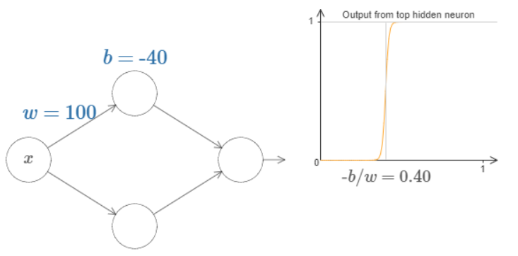
Fig. 16 \(s=−b/w\)
It will greatly simplify our lives to describe hidden neurons using just a single parameter, \(s\), which is the step position, \(s=−b/w\).
Up to now we’ve been focusing on the output from just the top hidden neuron. Let’s take a look at the behavior of the entire network. In particular, we’ll suppose the hidden neurons are computing step functions parameterized by step points \(s_1\) (top neuron) and \(s_2\) (bottom neuron). And they’ll have respective output weights \(w1\) and \(w2\). Here’s the network:
Fig. 17 What’s being plotted on the right is the weighted output \(w_1 a_1+w_2 a_2\) from the hidden layer. Here, \(a_1\) and \(a_2\) are the outputs from the top and bottom hidden neurons, respectively. These outputs are denoted with as because they’re often known as the neurons’ activations.
Note
By the way, that the output from the whole network is \(σ(w_1 a_1+w_2 a_2+b)\), where \(b\) is the bias on the output neuron. Obviously, this isn’t the same as the weighted output from the hidden layer, which is what we’re plotting here. We’re going to focus on the weighted output from the hidden layer right now, and only later will we think about how that relates to the output from the whole network.
Of course, we can rescale the bump to have any height at all. Let’s use a single parameter, \(h\), to denote the height. To reduce clutter we’ll also remove the \(s_1...\) and \(w_1...\) notations.
Fig. 18 Changing the value of \(h\) up and down, to see how the height of the bump changes
We can use our bump-making trick to get two bumps, by gluing two pairs of hidden neurons together into the same network. More generally, we can use this idea to get as many peaks as we want, of any height. In particular, we can divide the interval \([0,1]\) up into a large number, \(N\), of subintervals, and use \(N\) pairs of hidden neurons to set up peaks of any desired height. Let’s see how this works for \(N=5\).
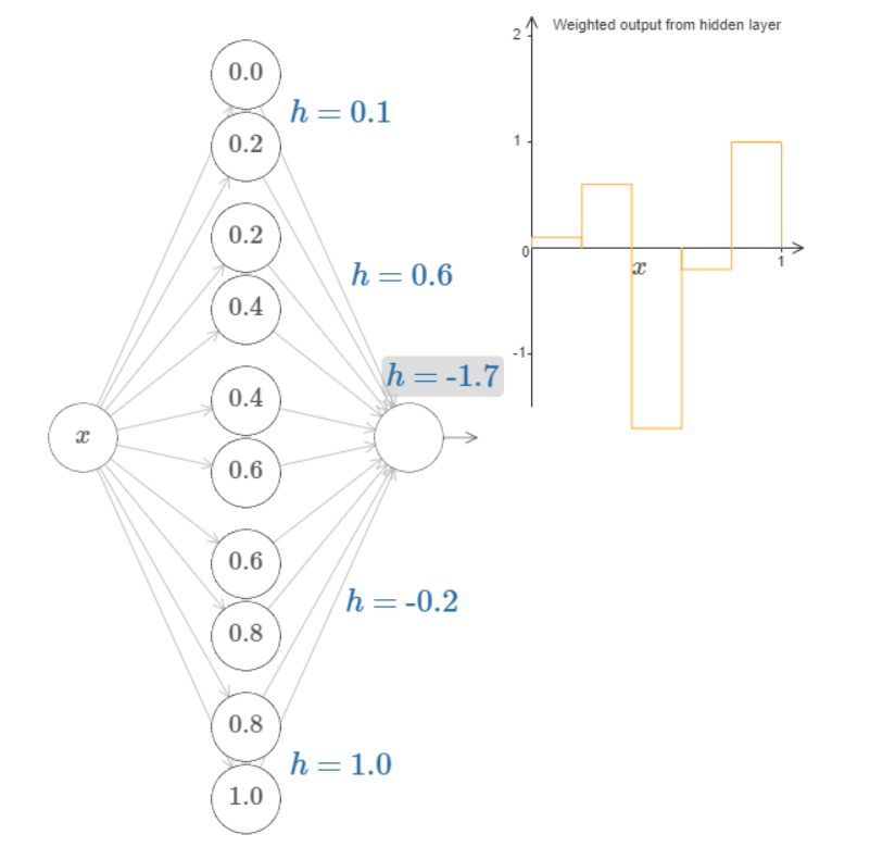
Fig. 19 You can see that there are five pairs of hidden neurons. The step points for the respective pairs of neurons are \(0,1/5\), then \(1/5,2/5\), and so on, out to \(4/5,5/5\). These values are fixed - they make it so we get five evenly spaced bumps on the graph.
Let’s think back to the function I plotted at the beginning of the chapter:
Fig. 20 The function is actually \(f(x)=0.2+0.4x^2+0.3xsin(15x)+0.05cos(50x)\) plotted over \(x\) from \(0\) to \(1\), and with the \(y\) axis taking values from \(0\) to \(1\).
That’s obviously not a trivial function. We are going to figure out how to compute it using a neural network.
In our networks above we’ve been analyzing the weighted combination \(\sum w_ja_j\) output from the hidden neurons. We now know how to get a lot of control over this quantity. But, as I noted earlier, this quantity is not what’s output from the network. What’s output from the network is \(σ(∑w_j a_j+b)\) where \(b\) is the bias on the output neuron. Is there some way we can achieve control over the actual output from the network?
The solution is to design a neural network whose hidden layer has a weighted output given by \(σ−1 \bullet f(x)\), where \(σ−1\) is just the inverse of the \(σ\) function. That is, we want the weighted output from the hidden layer to be:
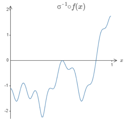
If we can do this, then the output from the network as a whole will be a good approximation to \(f(x)\).
Note
We have set the bias on the output neuron to 0.
We’ve now figured out all the elements necessary for the network to approximately compute the function \(f(x)\)! It’s only a coarse approximation, but we could easily do much better, merely by increasing the number of pairs of hidden neurons, allowing more bumps.
In particular, it’s easy to convert all the data we have found back into the standard parameterization used for neural networks. Let me just recap quickly how that works:
The first layer of weights all have some large, constant value, say \(w=1000\).
The biases on the hidden neurons are just \(b=−ws\). So, for instance, for the second hidden neuron s=0.2 becomes \(b=−1000×0.2=−200\).
The final layer of weights are determined by the \(h\) values. So, for instance, the value you’ve chosen above for the first \(h\), \(h= -0.9\), means that the output weights from the top two hidden neurons are \(-0.9\) and \(0.9\), respectively. And so on, for the entire layer of output weights.
Finally, the bias on the output neuron is \(0\).
That’s everything: we now have a complete description of a neural network which does a pretty good job computing our original goal function. And we understand how to improve the quality of the approximation by improving the number of hidden neurons.
What’s more, there was nothing special about our original goal function, \(f(x)=0.2+0.4x^2+0.3sin(15x)+0.05cos(50x)\). We could have used this procedure for any continuous function from \([0,1]\) to \([0,1]\). In essence, we’re using our single-layer neural networks to build a lookup table for the function. And we’ll be able to build on this idea to provide a general proof of universality.
Many input variables
The idea pitched above is appicable for 2 input variables as well, just that in that case there will be an increase in dimensionality.
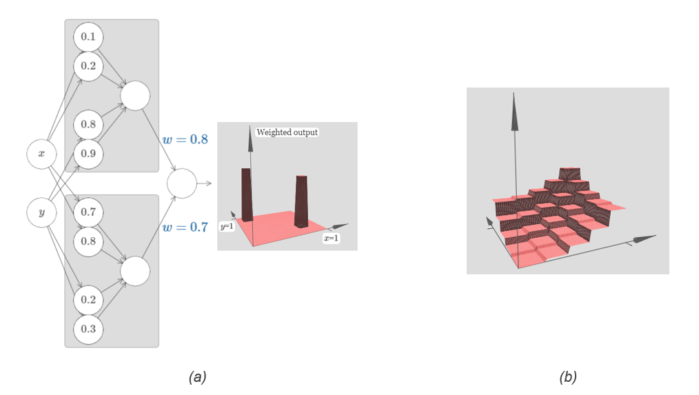
Fig. 23 (a) Bump changes to tower in higher dimension (b) Many such towers
By gluing together many such networks we can get as many towers as we want, and so approximate an arbitrary function of three variables. Exactly the same idea works in \(m\) dimensions. The only change needed is to make the output bias \((−m+1/2)h\), in order to get the right kind of sandwiching behavior to level the plateau.
Okay, so we now know how to use neural networks to approximate a real-valued function of many variables. What about vector-valued functions \(f(x_1,…,x_m)\epsilon R_n\)? Of course, such a function can be regarded as just \(n\) separate real-valued functions, \(f^1(x_1,…,x_m),f^2(x_1,…,x_m)\), and so on. So we create a network approximating \(f_1\), another network for \(f_2\), and so on. And then we simply glue all the networks together. So that’s also easy to cope with.
Extension beyond sigmoid neurons
We’ve proved that networks made up of sigmoid neurons can compute any function. Recall that in a sigmoid neuron the inputs \(x_1,x_2,…\) result in the output \(σ(∑w_jx_j+b)\), where \(w_j\) are the weights, \(b\) is the bias, and \(σ\) is the sigmoid function. What if we consider a different type of neuron, one using some other activation function, \(s(z)\)?
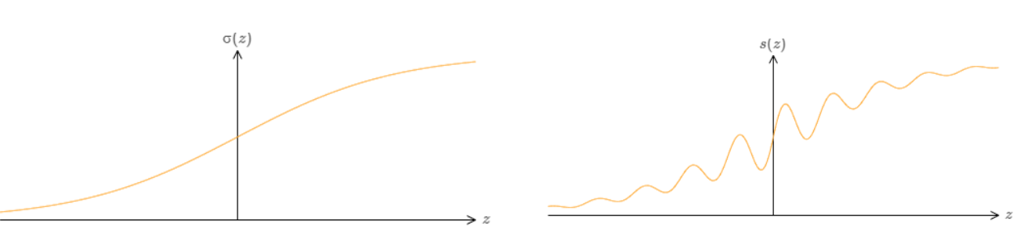
Fig. 24 \(σ\) vs \(s(z)\)
We can use this activation function to get a step function, just as we did with the sigmoid.
Fig. 25 Just as with the sigmoid, this causes the activation function to contract, and ultimately \(s(z)\) becomes a very good approximation to a step function.
What properties does s(z) need to satisfy in order for this to work?
We do need to assume that s(z) is well-defined as \(z→−∞\) and \(z→∞\). These two limits are the two values taken on by our step function.
We also need to assume that these limits are different from one another. If they weren’t, there’d be no step, simply a flat graph! But provided the activation function \(s(z)\) satisfies these properties, neurons based on such an activation function are universal for computation.
Note
Rectified Linear Unit(ReLU) does not satisfy the conditions just given for universality.
Fixing up the step functions
Up to now, we’ve been assuming that our neurons can produce step functions exactly. That’s a pretty good approximation, but it is only an approximation. In fact, there will be a narrow window of failure, illustrated in the following graph, in which the function behaves very differently from a step function:
In these windows of failure the explanation given for universality will fail. Now, it’s not a terrible failure. By making the weights input to the neurons big enough we can make these windows of failure as small as we like. Certainly, we can make the window much narrower than I’ve shown above - narrower, indeed, than our eye could see. So perhaps we might not worry too much about this problem.
Nonetheless, it’d be nice to have some way of addressing the problem.
In fact, the problem turns out to be easy to fix. Let’s look at the fix for neural networks computing functions with just one input and one output. The same ideas work also to address the problem when there are more inputs and outputs.
In particular, suppose we want our network to compute some function, f. As before, we do this by trying to design our network so that the weighted output from our hidden layer of neurons is \(σ^{−1}\dot f(x)\). If we were to do this using the technique described earlier, we’d use the hidden neurons to produce a sequence of bump functions:
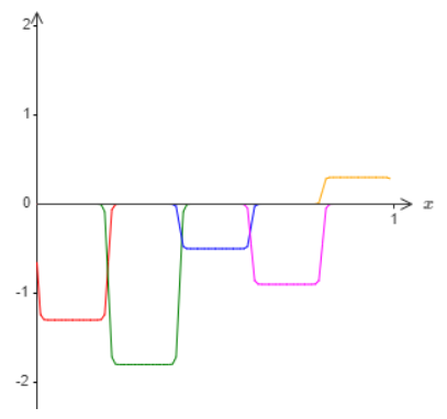
Again, I’ve exaggerated the size of the windows of failure, in order to make them easier to see. It should be pretty clear that if we add all these bump functions up we’ll end up with a reasonable approximation to \(σ−1\dot f(x)\), except within the windows of failure.
Suppose that instead of using the approximation just described, we use a set of hidden neurons to compute an approximation to half our original goal function, i.e., to \(σ^{−1}\dot f(x)/2\). Of course, this looks just like a scaled down version of the last graph:
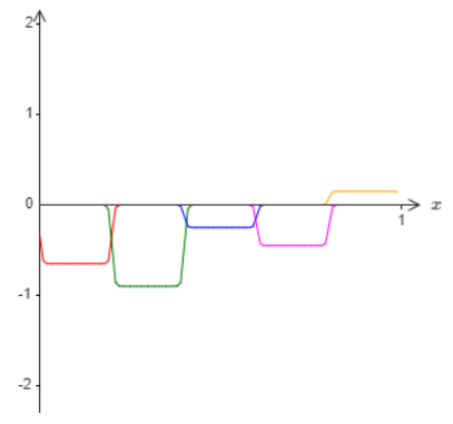
And suppose we use another set of hidden neurons to compute an approximation to \(σ^{−1}\dot f(x)/2\), but with the bases of the bumps shifted by half the width of a bump:
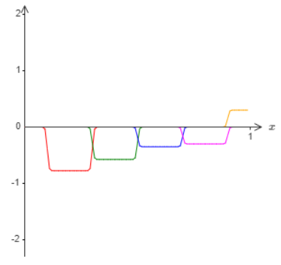
Now we have two different approximations to \(σ^{−1}\dot f(x)/2\). If we add up the two approximations we’ll get an overall approximation to \(σ^{−1}\dot f(x)\)). That overall approximation will still have failures in small windows. But the problem will be much less than before. The reason is that points in a failure window for one approximation won’t be in a failure window for the other. And so the approximation will be a factor roughly \(2\) better in those windows.
We could do even better by adding up a large number, \(M\), of overlapping approximations to the function \(σ^{−1}\dot f(x)/M\). Provided the windows of failure are narrow enough, a point will only ever be in one window of failure. And provided we’re using a large enough number \(M\) of overlapping approximations, the result will be an excellent overall approximation.
Conclusion
The explanation for universality we’ve discussed is certainly not a practical prescription for how to compute using neural networks! In this, it’s much like proofs of universality for NAND gates and the like. For this reason, I’ve focused mostly on trying to make the construction clear and easy to follow, and not on optimizing the details of the construction. However, you may find it a fun and instructive exercise to see if you can improve the construction.
Although the result isn’t directly useful in constructing networks, it’s important because it takes off the table the question of whether any particular function is computable using a neural network. The answer to that question is always “yes”. So the right question to ask is not whether any particular function is computable, but rather what’s a good way to compute the function.
The universality construction we’ve developed uses just two hidden layers to compute an arbitrary function. Furthermore, as we’ve discussed, it’s possible to get the same result with just a single hidden layer. Given this, you might wonder why we would ever be interested in deep networks, i.e., networks with many hidden layers. Can’t we simply replace those networks with shallow, single hidden layer networks?
While in principle that’s possible, there are good practical reasons to use deep networks. Deep networks have a hierarchical structure which makes them particularly well adapted to learn the hierarchies of knowledge that seem to be useful in solving real-world problems. Put more concretely, when attacking problems such as image recognition, it helps to use a system that understands not just individual pixels, but also increasingly more complex concepts: from edges to simple geometric shapes, all the way up through complex, multi-object scenes. Deep networks do a better job than shallow networks at learning such hierarchies of knowledge. To sum up: universality tells us that neural networks can compute any function; and empirical evidence suggests that deep networks are the networks best adapted to learn the functions useful in solving many real-world problems.
Code Snippet
import numpy as np
from keras.models import Sequential
from keras.layers import Dense
from sklearn.preprocessing import MinMaxScaler
from IPython.display import clear_output # to clear output before printing
import matplotlib.pyplot as plt

np.random.seed(7)
X = np.linspace(0.0 , 2.0 * np.pi, 10000).reshape(-1, 1)
Y = np.sin(X)
x_scaler = MinMaxScaler()
y_scaler = MinMaxScaler()
X = x_scaler.fit_transform(X)
Y = y_scaler.fit_transform(Y)

def plotgraph(X, Y, res,i): # to plot the graph
    plt.plot(X, res, label = "predicted")
    plt.plot(X, Y, label = "true")
    plt.title("Epoch Count: " + str(i))
    plt.legend()
    plt.show()

for i in range(0,10): # for loop is needed just to visualize the training progress, it can be removed

    model = Sequential()
    model.add(Dense(50, input_dim=X.shape[1], activation='relu'))
    model.add(Dense(50, input_dim=X.shape[1], activation='relu'))
    model.add(Dense(1, activation='linear'))
    model.compile(loss='mse', optimizer='adam', metrics=['mae'])
    model.fit(X, Y, epochs=i, batch_size=32, verbose=0)
    res = model.predict(X, batch_size=32)
    res_rscl = y_scaler.inverse_transform(res)
    Y_rscl = y_scaler.inverse_transform(Y)
    plotgraph(X, Y, res, i)
    clear_output(wait=True)
Fig. 30 A Neural Network slowly approximating the Sine function