Hypothesis Testing
Contents
Hypothesis Testing#
Inferential Statistics#
Sometimes, you may require a very large amount of data for your analysis which may need too much time and resources to acquire. In such situations, you are forced to work with a smaller sample of the data, instead of having the entire data to work with.
Situations like these arise all the time at big companies like Amazon. For example, say the Amazon QC department wants to know what proportion of the products in its warehouses are defective. Instead of going through all of its products (which would be a lot!), the Amazon QC team can just check a small sample of 1,000 products and then find, for this sample, the defect rate (i.e. the proportion of defective products). Then, based on this sample’s defect rate, the team can “infer” what the defect rate is for all the products in the warehouses. This process of “inferring” insights from sample data is called “Inferential Statistics”.
Hypothesis Testing#
Hypothesis testing is used to confirm your conclusions about the population parameter. Through this we can conclude if there is enough evidence to confirm the hypothesis about the population.
\(H_0 =\) null hypothesis, what is already present; always has the following signs: = OR ≤ OR ≥
\(H_1 =\) alternate hypothesis, a challenge to the null hypothesis; always has the following signs: ≠ OR > OR <
Steps#
There is an initial research hypothesis of which the truth is unknown.
The first step is to state the relevant null and alternative hypotheses. This is important, as mis-stating the hypotheses will muddy the rest of the process.
The second step is to consider the statistical assumptions being made about the sample in doing the test; for example, assumptions about the statistical independence or about the form of the distributions of the observations. This is equally important as invalid assumptions will mean that the results of the test are invalid.
Decide which test is appropriate, and state the relevant test statistic \(T\).
Derive the distribution of the test statistic under the null hypothesis from the assumptions. In standard cases this will be a well-known result. For example, the test statistic might follow a Student’s t distribution with known degrees of freedom, or a normal distribution with known mean and variance. If the distribution of the test statistic is completely fixed by the null hypothesis we call the hypothesis simple, otherwise it is called composite.
Select a significance level (\(\alpha\)), a probability threshold below which the null hypothesis will be rejected. Common values are \(5\%\) and \(1\%\).
The distribution of the test statistic under the null hypothesis partitions the possible values of T into those for which the null hypothesis is rejected—the so-called critical region—and those for which it is not. The probability of the critical region is \(\alpha\). In the case of a composite null hypothesis, the maximal probability of the critical region is \(\alpha\).
Compute from the observations the observed value \(t_{obs}\) of the test statistic \(T\).
Decide to either reject the null hypothesis in favor of the alternative or not reject it. The decision rule is to reject the null hypothesis \(H_0\) if the observed value \(t_{obs}\) is in the critical region, and not to reject the null hypothesis otherwise.
A common alternative formulation of this process goes as follows:
Compute from the observations the observed value tobs of the test statistic \(T\).
Calculate the \(p\)-value. This is the probability, under the null hypothesis, of sampling a test statistic at least as extreme as that which was observed (the maximal probability of that event, if the hypothesis is composite).
Reject the null hypothesis, in favor of the alternative hypothesis, if and only if the \(p\)-value is less than (or equal to) the significance level (the selected probability) threshold (\(\alpha\)), for example \(0.05\) or \(0.01\).
The former process was advantageous in the past when only tables of test statistics at common probability thresholds were available. It allowed a decision to be made without the calculation of a probability. It was adequate for classwork and for operational use, but it was deficient for reporting results. The latter process relied on extensive tables or on computational support not always available. The explicit calculation of a probability is useful for reporting. The calculations are now trivially performed with appropriate software.
The difference in the two processes applied to the Radioactive suitcase example (below):
“The Geiger-counter reading is \(10\). The limit is \(9\). Check the suitcase.”
“The Geiger-counter reading is high; \(97\%\) of safe suitcases have lower readings. The limit is \(95\%\). Check the suitcase.”
The former report is adequate, the latter gives a more detailed explanation of the data and the reason why the suitcase is being checked.
Example#
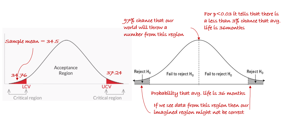
A manufacturer claims that the average life of its products is \(36\) months. An auditor selects a sample of \(49\) units of the product and calculates the average life to be \(34.5\) months. The population standard deviation is \(4\) months. Test the manufacturer’s claim at \(3\%\) significance level.
So as per the above problem:
\(H_0 : \mu = 36\) months
\(H_1 : \mu ≠ 36\) months
\(\alpha = 3\%\) or \(0.03\) \(\sigma = 4\) \(N = 49\)
First we will take a look into the Critical-value method:
In this case we will have critical region at both sides with total area of \(0.03\).
So the area to the right = \(0.015\), which means that area till UCV (cumulative probability till that point) \(= 1-0.015=0.985\)
\(z\)-score of cumulative probability of UCV (\(Z_c\) in this case) \(= z\)-score of \(0.985 = 2.17\)
Calculating the critical values UCV/LCV \(= \mu \pm Z_c * \frac{\sigma}{\sqrt{N}} \)
UCV/LCV \(= 36 \pm 2.17 * \frac{4}{\sqrt{49}} = 37.24 \text{ and } 34.76\)
Now as the sample mean \(34.5\) is not between UCV and LCV hence we reject the null hypothesis.
Now let’s solve it using the \(p\)-value method:
Calculate the \(z\)-score of \(34.5 = \frac{\bar{x} -\mu}{\frac{\sigma}{\sqrt{N}}} = -2.62\)
Calculate the p-value from table \(= 0.0044\), which is cumulative area till sample point$
As this it is in the left hand side hence there is no need to substract from \(1\).
Now this will be a 2-tailed test as we are checking for inequality, we need to multiply by \(2 = 0.0088\), remember 1-tailed test provides more power to detect an effect because the entire weight is allocated to one direction only.
As \(p\)-value is \(< \alpha\) so we reject null-hypothesis.
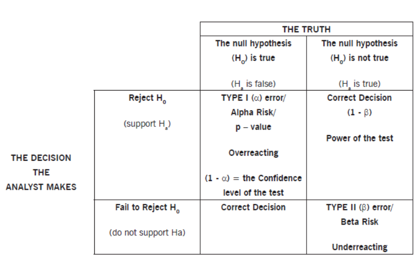
Errors in Hypothesis Testing#
Questions#
Problem: Limitations of p-value
Can you tell some limitations of p-value?
Solution:
Some limitations of p-value are as follows:
p-value does not give the probability of how true the null hypothesis was. It just gives a binary decision on if it can be rejected or not
p-value does not consider how precise the effect is (as it assumes we know the sample size, does not tell much about sample size)
Problem: [AMAZON] Testing Hypotheses with t-Test
You are testing hundreds of hypotheses with a t-test, what considerations should be made?
Solution:
Type 1 error will scale the more the number of t-tests are run. If \(\alpha = 0.05\) then there is \(5%\) chance of Type 1 error on a single test, then across many tests \(p(Type I)\) will increase. For example with 2 tests:
\( P(\text{type I error}) = p(\text{type I error on A OR type I error on B}) \) \( = 2p(\text{type I error on single test}) - p(\text{type I error on A AND type I error on B}) \) \( = 2*.05 - .05^2 (\text{assuming independence of tests}) = 0.5 - .025 = .075 \)
If you want your \(p(type I error)\) across n-tests to remain at \(5%\), you will need to decrease the $\alpha\ in each individual test. Bonferroni correction can be applied. Basically alpha will be reduced to alpha/n. n is number of experiments you are running.
Otherwise, you can try and run an F-test to start in order to identify if a least \(1\) test sees some significant effect. Then run a t-test on the specific experiment with the highest effect size. Granted, the p-value of the test will also depend on the variance of the sample in the given test, if we assume constant variance across tests, then the test with the highest effect size is in expectation the best performing test. Only running a single t-test will keep your p(type I error) low.
Problem: Selection Bias
Explain selection bias (with regard to a dataset, not variable selection). Why is it important? How can data management procedures such as missing data handling make it worse?
Solution:
Selection bias is the phenomenon of selecting individuals, groups or data for analysis in such a way that proper randomization is not achieved, ultimately resulting in a sample that is not representative of the population. Understanding and identifying selection bias is important because it can significantly skew results and provide false insights about a particular population group. Types of selection bias include:
sampling bias: a biased sample caused by non-random sampling
time interval: selecting a specific time frame that supports the desired conclusion. e.g. conducting a sales analysis near Christmas.
exposure: includes clinical susceptibility bias, protopathic bias, indication bias. Read more here.
data: includes cherry-picking, suppressing evidence, and the fallacy of incomplete evidence.
attrition: attrition bias is similar to survivorship bias, where only those that ‘survived’ a long process are included in an analysis, or failure bias, where those that ‘failed’ are only included
observer selection: related to the Anthropic principle, which is a philosophical consideration that any data we collect about the universe is filtered by the fact that, in order for it to be observable, it must be compatible with the conscious and sapient life that observes it.
Handling missing data can make selection bias worse because different methods impact the data in different ways. For example, if you replace null values with the mean of the data, you adding bias in the sense that you’re assuming that the data is not as spread out as it might actually be.