Regression
Contents
Regression#
Linear Regression#
\(Y = b_0 + b_1 * x_1 + b_2 * x_2 + \epsilon\)
The idea is to find the line or plane which best fits the data. Collectively, \(b_0, b_1, b_2\) are called regression coefficients. \(\epsilon\) is the error term, the part of \(Y\) the regression model is unable to explain.
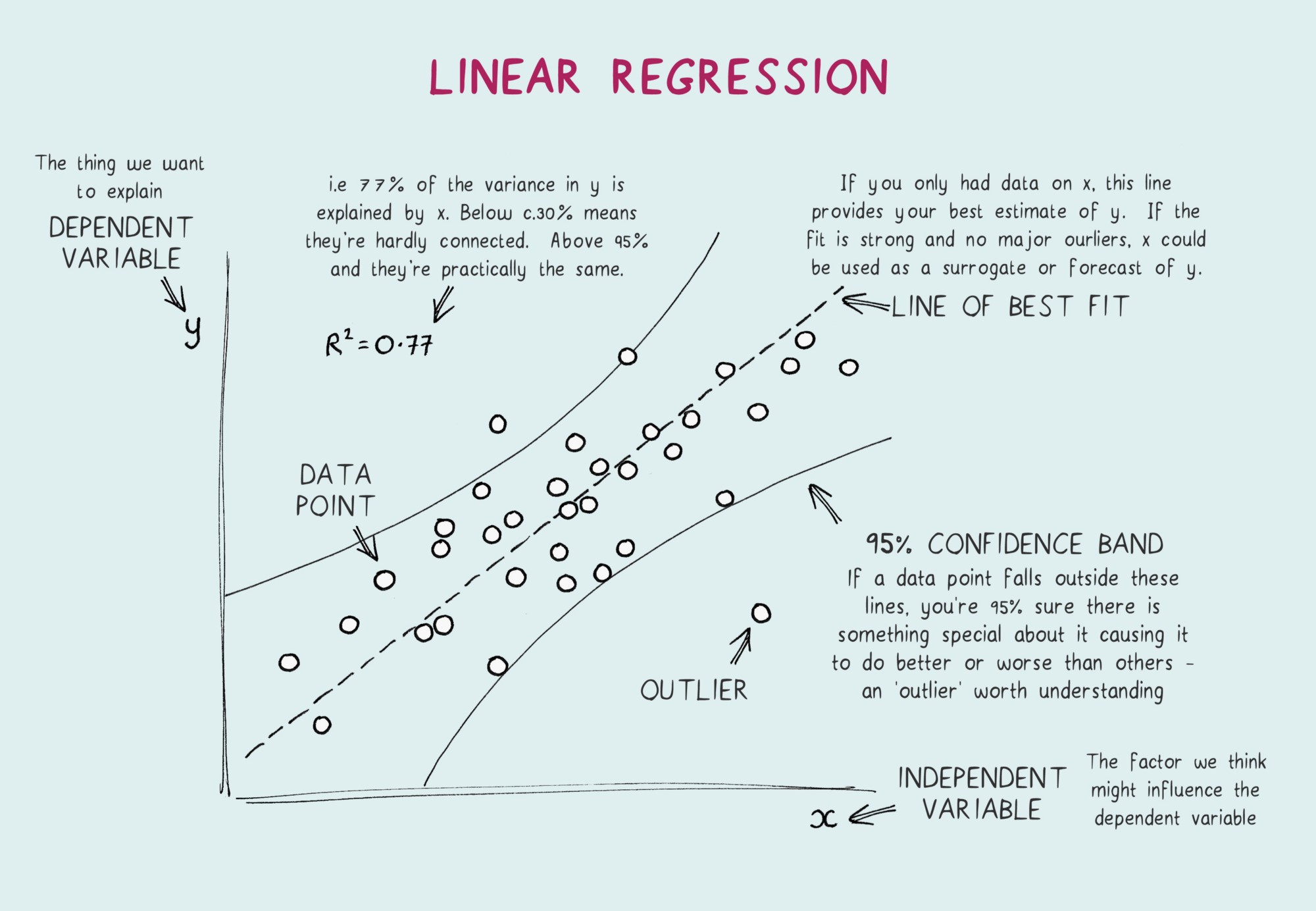
Metrics#
Now once you have the model fit next comes the metrics to measure how good the fit is, some of the common metrics are as follows:
\(RSS\) (Residual sum of squares) \(= (Y_{actual} - Y_{predicted})^2\), it changes with scale change
\(TSS\) (Total sum of squares) \(= (Y_{actual} - Y_{avg})^2\)
\(R^2\) \(= 1-\frac{RSS}{TSS} \), more the better, increases with more coefficients
\(RSE\) (Residual Standard Error) \( = \sqrt{\frac{RSS}{d.o.f}}\), here \(d.o.f = n-2\)
Feature selection#
Hypothesis testing and using p-values to understand if the feature is important or not
Using metrics like \(\text{Adjusted} R^2\), \(AIC\), \(BIC\), etc. which takes into consideration the number of features used to build the model and penalizes accordingly
How do we find the model that minimizes a metric like \(AIC\)? One approach is to search through all possible models, called all subset regression. This is computationally expensive and is not feasible for problems with large data and many variables. An attractive alternative is to use stepwise regression about which we learned above, this successively adds and drops predictors to find a model that lowers \(AIC\). Simpler yet are forward selection and backward selection. In forward selection, you start with no predictors and add them one-by-one, at each step adding the predictor that has the largest contribution to , stopping when the contribution is no longer statistically significant. In backward selection, or backward elimination, you start with the full model and take away predictors that are not statistically significant until you are left with a model in which all predictors are statistically significant.
Penalized Regression or Regularization:
Penalized regression is similar in spirit to AIC. Instead of explicitly searching through a discrete set of models, the model-fitting equation incorporates a constraint that penalizes the model for too many variables (parameters). Rather than eliminating predictor variables entirely — as with stepwise, forward, and backward selection — penalized regression applies the penalty by reducing coefficients, in some cases to near zero. Common penalized regression methods are ridge regression and lasso regression. Regularization is nothing but adding a penalty term to the objective function and control the model complexity using that penalty term. It can be used for many machine learning Algorithms. Both Ridge and Lasso regression uses \(L2\) and \(L1\) regularizations.
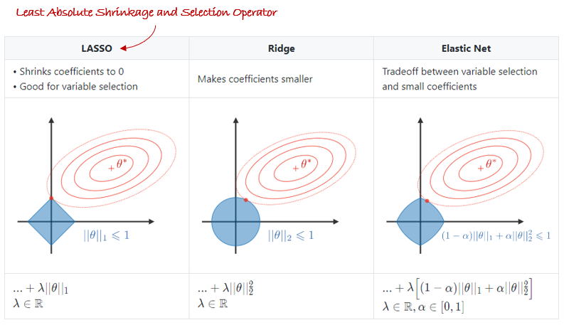
Note
Ridge brings the coefficients close to \(0\) but not exactly to \(0\) which results in the model retaining all the features. Lasso on the other hand brings the coefficients to \(0\) hence results in reduced features. Lasso shrinks the coefficients by same amount whereas Ridge shrinks them by same proportion.
Elastic Net is another useful techniques which combines both L1 and L2 regularization.
Assumptions#
The relationship between \(X\) and \(Y\) is linear. Because we are fitting a linear model, we assume that the relationship really is linear, and that the errors, or residuals, are simply random fluctuations around the true line.
The error terms are normally distributed. This can be checked with a Q-Q plot
Error terms are independent of each other. This can be checked with a ACF plot. This can be used while checking independence while using a time-series data
Error terms are homoscedastic, i.e. they have constant variance. Residulas Vs Fitted graph should be flat. This means that the variability in the response is changing as the predicted value increases. This is a problem, in part, because the observations with larger errors will have more pull or influence on the fitted model.
The independent variables are not multicollinear. Multicollinearity is when a variable can be explained as a combination of other variables. This can be checked by using VIF(Variance inflation factor) \(= \frac{1}{1-R_i^2}\).
A VIF score of \(>10\) indicates there there is a problem
If a multicollinear variable is present the coefficients swing wildly thereby affecting the interpretability of the model. P-vales are not reliable. But it doesnot affect prediction or the goodness of fit statistics.
To deal with multicollinearity
drop variables
create new features from existing ones
PCA/PLS
Note
One very important point to remember is that Generalized Linear Regression is called so because \(Y\) is linear w.r.t its coefficients \(b_0, b_1, b_2\), etc. it is irrespective of whether the features \(x_1, x_2\), etc. are linear or not. Meaning \(x_1\) can actually be \(x_1^2\) and it won’t matter.
Non-Linear Regression#
In some cases, the true relationship between the outcome and a predictor variable might not be linear. There are different solutions extending the linear regression model for capturing these nonlinear effects, some of these are covered below.
Polynomial Regression#
The equation of polynomial becomes something like this.
\(Y = b_0 + b_1 * x_1 + b_2 * x_1^2 + b_n * x_1^n \) and so on…
The degree of order which to use is a Hyperparameter, and we need to choose it wisely. But using a high degree of polynomial tries to overfit the data and for smaller values of degree, the model tries to underfit so we need to find the optimum value of a degree. Polynomial Regression on datasets with high variability chances to result in over-fitting.
Regression Splines#
In order to overcome the disadvantages of polynomial regression, we can use an improved regression technique which, instead of building one model for the entire dataset, divides the dataset into multiple bins and fits each bin with a separate model. Such a technique is known as Regression spline.
In polynomial regression, we generated new features by using various polynomial functions on the existing features which imposed a global structure on the dataset. To overcome this, we can divide the distribution of the data into separate portions and fit linear or low degree polynomial functions on each of these portions. The points where the division occurs are called Knots. Functions which we can use for modelling each piece/bin are known as Piecewise functions. There are various piecewise functions that we can use to fit these individual bins.
Generalized additive models#
It does the same thing as above but just removes the need to specifying the knots. It fits spline models with automated selection of knots.
Questions#
Problem: [UPSTART] Regression Coefficient
Suppose we have two variables, \(X\) and \(Y\), where \(Y = X +\) some normal white noise.
What will our coefficient be of we run a regression of \(Y\) on \(X\)?
What happens if we run a regression of \(X\) on \(Y\)?
Solution:
Let’s start with \(Y = X\), then the regression line is a perfect fit. The points of such a dataset is \((1,1),(2,2),(3,3),(4,4),(5,5)\)
Adding some normal white noise to these points \((1,1),(2,3),(3,5),(4,5),(5,5)\). A regression line fit on these points will move up. Hence the coefficients of \(Y = mX+c\), \(m\) will increase, \(c\) might still stay at \(0\) or at max increase.
This movement will go in the negative direction if we predict \(X\) based on \(Y\)
Problem: Linear Regression in Time Series
Do you think Linear Regression should be used in Time series analysis?
Solution:
Linear Regression as per me can be used in Time Series but might not always give good results. Few reasons which come up are:
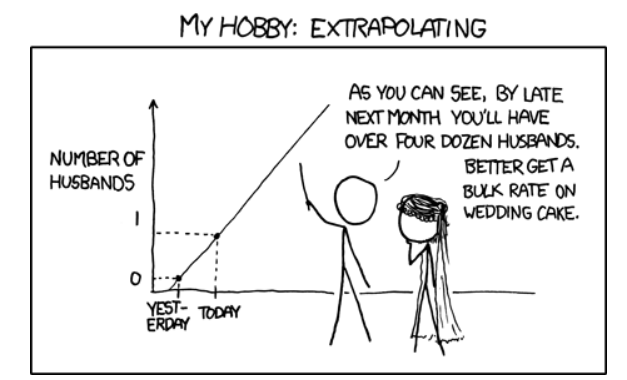
Linear Regression is good for intrapolation but not for extrapolation so the results can vary wildly
When Linear Regression is used but observations are correlated (as in time series data) you will have a biased estimate of the variance
Moreover, time-series data have a pattern, such as during peak hours, festive seasons, etc., which would most likely be treated as outliers in the linear regression analysis
Problem: [AIRBNB] Booking Regression
Let’s say we want to build a model to predict booking prices.
Explain the difference between a linear regression versus a random forest regression.
Which one would likely perform better?
Solution:
Linear Regression is used to predict continuous outputs where there is a linear relationship between the features of the dataset and the output variable. It is used for regression problems where you are trying to predict something with infinite possible answers such as the price of a house.
In the case of regression, decision trees in random forest learn by splitting the training examples in a way such that the sum of squared residuals is minimized. To classify a new object based on attributes, each tree gives a classification and we say the tree “votes” for that class. The forest chooses the classification having the most votes (over all the trees in the forest) and in case of regression, it takes the average of outputs by different trees. It is useful when there are complex relationships between the features and the output variables. They also work well compared to other Algorithms when there are missing features, when there is a mix of categorical and numerical features and when there is a big difference in the scale of features.
It is difficult to tell which will perform better, it completely depends on the problem statement and the available data. Other than the points mentioned above some of the Key advantages of linear models over tree-based ones are:
they can extrapolate (e.g. if labels are between 1-5 in train set, tree based model will never predict 10, but linear will)
could be used for anomaly detection because of extrapolation
interpretability (yes, tree based models have feature importance, but it’s only a proxy, weights in linear model are better)
need less data to get good results
Random Forest is able to discover more complex relation at the cost of time
The first point becomes clearly important in this case as we would need booking price values which might not necessarily be in the training data range.
Problem: [GOOGLE] Adding Noise
Say we are running a probabilistic linear regression which does a good job modeling the underlying relationship between some \(y\) and \(x\). Now assume all inputs have some noise \(\epsilon\) added, which is independent of the training data.
What is the new objective function? How do you compute it?
Solution:
The objective function for linear regression where \(x\) is set of input vectors and \(w\) are the weights: \(L(w) = E[(w^Tx-y)^2]\)
Let’s assume that the noise added is Gaussian as follows: \(\epsilon \sim N(0, \lambda I)\), then the new objective function is given by:\(L(w) = E[(w^T(x + \epsilon)-y)^2]\).
To compute it, we simplify: \(L'(w) = E[(w^T x -y + w^T\epsilon)^2]\) \(L'(w) = E[(w^T x - y)^2 + 2(w^Tx-y)w^T\epsilon +w^T\epsilon \epsilon^Tw]\) \(L'(w) = E[(w^T x - y)^2] + E[2(w^Tx-y)w^T\epsilon] + E[w^T\epsilon \epsilon^Tw]\)
We know that the expectation for \(\epsilon\) is \(0\) so the middle term becomes \(0\) and we are left with:\(L'(w) = L(w) + 0 + w^TE[\epsilon \epsilon^T]w\)
The last term can be simplified as: \(L'(w) = L(w) + w^T\lambda Iw\)
And therefore the objective function simplifies to that of L2-regularization: \(L'(w) = L(w) + \lambda||w||^2\)
Problem: [UBER] L1 vs L2
What is L1 and L2 regularization? What are the differences between the two?
Solution:
\(L1\) and \(L2\) regularization are both methods of regularization that attempt to prevent overfitting in machine learning. For a regular regression model assume the loss function is given by \(L\). \(L1\) adds the absolute value of the coefficients as a penalty term, whereas \(L2\) adds the squared magnitude of the coefficients as a penalty term.
The loss function for the two are:
\(Loss(L_1) = L + \lambda |w_i| \)
\(Loss(L_2) = L + \lambda |w_i^2| \)
Where the loss function \(L\) is the sum of errors squared, given by the following, where \(f(x)\) is the model of interest, for example, linear regression with \(p\) predictors:
\(L = \sum_{i=1}^{n} (y_i - f(x_i))^2 = \sum_{i=1}^{n} (y_i - \sum_{j=1}^{p}(x_{ij}w_j) )^2 \space \text{for linear regression}\)
If we run gradient descent on the weights \(w\), we find that \(L1\) regularization will force any weight closer to \(0\), irrespective of its magnitude, whereas, for the \(L2\) regularization, the rate at which the weight goes towards \(0\) becomes slower as the rate goes towards \(0\). Because of this, \(L1\) is more likely to “zero” out particular weights, and hence removing certain features from the model completely, leading to more sparse models.
Problem: [TESLA] Choice of Cost Function
You’re working with several sensors that are designed to predict a particular energy consumption metric on a vehicle. Using the outputs of the sensors, you build a linear regression model to make the prediction. There are many sensors, and several of the sensors are prone to complete failure.
What are some cost functions you might consider, and which would you decide to minimize in this scenario?
Solution:
There are two potential cost functions here, one using the \(L1\) norm and the other using the \(L2\) norm. Below are two basic cost functions using an L1 and L2 norm respectively:
\(J(w) = ||Xw-y||\)
\(J(w) = |Xw-y|^2\)
It would be more sensible to use an \(L1\) norm in this case since the \(L1\) norm penalizes the outliers harder and thus gives less weight to the complete failures than the \(L2\) norm does.
Additionally, it would be prudent to involve a regularization term to account for noise. If we assume that the noise added to each sensor uniformly as follows: \(\epsilon \sim N(0, \lambda I)\) then using traditional \(L2\) regularization, we would have the cost function: \(J(w) = ||Xw-y|| + \lambda||w||^2\)
However, given the fact that there are many sensors (and a broad range of how useful they are), we could instead assume that noise is added by: \(\epsilon \sim N(0, \lambda D)\) where each diagonal term in the matrix D represents the error term used for each sensor (and hence penalizing certain sensors more than others). Then our final cost function is given by: \(J(w) = ||Xw-y|| + \lambda w^TDw\)
Problem: [AIRBNB] Prove that maximizing the likelihood is equivalent to minimizing the sum of squared residuals
Suppose you are running a linear regression and model the error terms as being normally distributed. Show that in this setup, maximizing the likelihood of the data is equivalent to minimizing the sum of squared residuals.
Solution:
A mathematical derivation like this requires us to:
Define correct Mathematical symbols and their relationships through equations
Recall and use the definitions of the terms like likelihood and normally distributed
Perform Mathematical manipulation to derive the required result
Problem Setup:
A linear regression model proposes that the output \(y\) is linearly dependent on the input vector \(X\) by the relation,
\(y = W^T X + \beta\)
Where, \(X\) is an \(m\)-dimensional vector, and \((W; \beta) = \{w_1, w_2, ..., w_m; \beta\}\) are the parameters of the model.
Next, we are give a set of training data points, consisting of
a set of input vectors, \(X = \{X_1, X_2, ..., X_n\}\). Note that every input \(X_i\) is a vector, \(X_i = \{X_{i1}, X_{i2}, ..., X_{im}\}\)
and a set of outputs \(Y = \{y_1, y_2, ..., y_n\}\)
Given the values of the parameters \(W\) and \(\beta\), the estimate \(\hat{y}\) is given by
\(\hat{y}_i = \sum_{j=1}^m X_{ij} * w_j + \beta = X_{i1} * w_1 + X_{i2} * w_2 + ... + X_{im} * w_m + \beta \).
Finally, the error term for \(i^{th}\) input is simply the difference between the observed value \(y\) and the estimate \(\hat{y}\).
\(\epsilon_i(W, \beta) = y_i - \hat{y}_i = y_i - \sum_{j=1}^m X_{ij} * w_j - \beta\)
Note that the error term depends on the parameters of the model \(W\) and \(\beta\), and hence is denoted as \(\epsilon_i(W, \beta)\).
Likelihood:
Take a look at the problem statement again. We are assuming that the error terms are normally distributed. There is an implicit assumption that all the error terms are independent of each other. (Make sure you make this assumption explicit to your interviewer).
What does it mean for the error term to be normally distributed. It means that, by definition, the probability distribution function of the \(i^{th}\) error term is given by
\(l(\epsilon_i|W; \beta) = \frac{1}{\sqrt{2\pi}\sigma}exp\{\frac{-\epsilon_i^2}{2\sigma^2}\}\)
This probability distribution function of the \(i^{th}\) input is also called its likelihood function, and also depends on the parameters of the model, \(W\) and \(\beta\).
Since we are assuming that the error terms are also independent, their joint probability distribution, is given by the product of their likelihood.
\(l = \displaystyle \prod_{i=1}^n l(\epsilon_i|W; \beta)\) \( = \displaystyle \prod_{i=1}^n \frac{1}{\sqrt{2\pi}\sigma}exp\{\frac{-\epsilon_i^2}{2\sigma^2}\}\) \( = \displaystyle \frac{1}{(\sqrt{2\pi}\sigma)^n} \prod_{i=1}^n exp\{\frac{-\epsilon_i^2}{2\sigma^2}\}\) \( = \displaystyle \frac{1}{(\sqrt{2\pi}\sigma)^n} \prod_{i=1}^n exp\{\frac{-(y_i - \sum_{j=1}^m X_{ij} * w_j - \beta)^2}{2\sigma^2}\}\)
Maximum Likelihood Estimator:
The maximum likelihood estimator seeks to maximize the likelihood function defined above. For the maximization,
We can ignore the constant \(\frac{1}{(\sqrt{2\pi}\sigma)^n}\)
We can also take the log of the likelihood function, converting the product into sum
The log likelihood function of the errors is given by
\(L = log(l)\) \( = \displaystyle log(\prod_{i=1}^n exp\{\frac{-(y_i - \sum_{j=1}^m X_{ij} * w_j - \beta)^2}{2\sigma^2}\})\) \( = \displaystyle \sum_{i=1}^n {\frac{-(y_i - \sum_{j=1}^m X_{ij} * w_j - \beta)^2}{2\sigma^2}}\)
As a final step, for the purpose of optimization, we can ignore the constant multiplier \(2\sigma^2\) from the summation, giving us
\(L = \displaystyle \sum_{i=1}^n -(y_i - \sum_{j=1}^m X_{ij} * w_j - \beta)^2\)
But this is just the negative of the sum of squared errors!
Thus, if you want to maximize the likelihood (or log likelihood) of the errors, you better minimize the sum of squared errors of the estimates.