Recurrent Neural Network

Warning

This page is a work in progress

Normal neural network is insufficient to train sequence data. Some examples of sequence data are:

• Time series

• Music

• Videos

• Text

Sequential data contains multiple entities​ and the order in which these entities are present is important.

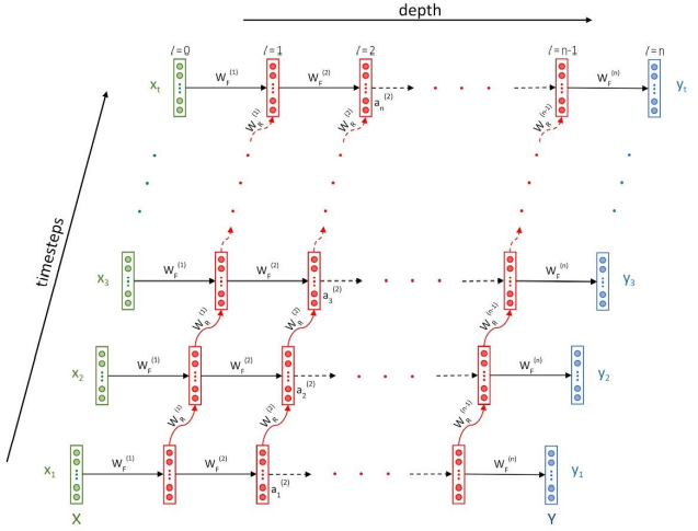
In RNN each activation is dependent on two things: the activation in the previous layer \(l-1\) at the current timestep \(t\), and the activation in the same layer \(l\) at the previous timestep \(t-1\)

Types of RNN

• Many to One: This architecture involves a sequence as an input and a single entity as an output​. E.g: next word prediction

• Many to Many: Model data which involves sequences in the input as well as the output​. Both the input and output sequences must have a one-to-one correspondence ​and therefore the input and output sequences are equal in length​. E.g: POS tagging of sentences

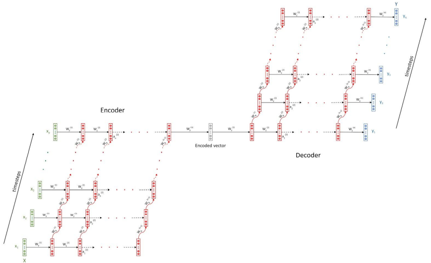
• Encoder-decoder: Here the length of the input and the output sequence is not equal​. It is used in problems such as language translation and document summarization. Here the errors are backpropagated from the decoder to the encoder. The encoder and decoder have a different set of weights and they are different RNNs altogether. The loss is calculated at each timestep which can either be backpropagated at each timestep, or the cumulative loss (sum of all the losses from all the timesteps of a sequence) can be backpropagated after the entire sequence is ingested. Generally, the errors are backpropagated once an RNN ingests an entire batch

• One to Many: This type of architecture has a single entity as an input and a sequence as the output​. It is used for generation such as music generation, creating drawings, generating text, etc.

Backpropagation Through Time (BPTT)

Any given term in an RNN depends not only on the current input but also on the input from previous timesteps​. The gradients not only flow back from the output layer to the input layer, but they also flow back in time from the last timestep to the first timestep. Hence the name backpropagation through time.

Exploding and Vanishing gradient:

• Vanishing: The vanishing gradient problem describes a situation encountered in the training of neural networks where the gradients used to update the weights shrink exponentially. As a consequence, the weights are not updated anymore, and learning stalls.

• Exploding: The exploding gradient problem describes a situation in the training of neural networks where the gradients used to update the weights grow exponentially. This prevents the backpropagation algorithm from making reasonable updates to the weights, and learning becomes unstable.

How to understand

• Vanishing:

  • The parameters of the higher layers change significantly whereas the parameters of lower layers would not change much (or not at all)

  • The model weights may become 0 during training

  • The model learns very slowly and perhaps the training stagnates at a very early stage just after a few iterations

• Exploding:

  • There is an exponential growth in the model parameters

  • The model weights may become NaN during training

  • The model experiences avalanche learning

How to rectify

• Use the ReLU Activation Function over the sigmoid activation function as it is prone to creating vanishing gradients, especially when several of them are chained together. This is due to the fact that the sigmoid function saturates towards 0 for large negative or towards 1 for large positive values.

• Another way to address vanishing and exploding gradients is through weight initialization techniques. In a neural network, we initialize the weights randomly. Certain techniques such as He initialization and Xavier initialization ensure that the weights are close to 1.

• Another simple option is gradient clipping. This way, you just define an interval within which you expected the gradients to fall. If the gradients exceed the permissible maximum, you automatically set them to the maximum upper bound of your interval. Similarly, if they fall below the permissible minimum, you automatically set them to the lower bound.

• To get rid of the vanishing gradients problem, the researchers came up with another type of cell that can be used inside an RNN layer, called the LSTM cell. We will take a look into that later.

Bidirectional RNNs

There are two kinds of problems in sequences:

• Offline sequences​: These allow for a lookahead in time. The entire sequence is present for your perusal. For example, a document present in your local drive where you have access to the entire document.

• Online sequences​: These don’t allow for a lookahead. For example, a person is speaking and you need to transcribe the speech. In this case, you don’t know what is going to come next.

You can make use of offline sequences by looking ahead. You can feed the offline sequences to an RNN in regular order as well as the reverse order to get better results in whatever task you’re doing. Such an RNN is called a bidirectional RNN​. In a bidirectional RNN, the input at each timestep is a concatenation of the entity present in regular order and the entity present in reverse order. For example, for a sentence of length \(100\), the input at the first timestep will be a concatenation of the first word \(x_1\) and the last word \(x_{100}\). A bidirectional RNN has \(2\)x number of parameters​ than a vanilla RNN.

LSTM